tick.prox
This module proposes a large number of proximal operator, allowing the use
many penalization techniques for model fitting. Namely, most optimization
problems considered in tick (but not all) can be written as
where \(f\) is a goodness-of-fit term and \(g\) is a function penalizing \(w\). Depending on the problem, you might want to use some function \(g\) in order to induce a specific property of the weights \(w\) of the model.
The proximal operator of a convex function \(g\) at some point \(w\) is defined as the unique minimizer of the problem
where \(t > 0\) is a regularization parameter and \(\| \cdot \|_2\) is the Euclidean norm. Note that in the particular case where \(g(w) = \delta_{C}(w)\), with \(C\) a convex set, then \(\text{prox}_g\) is a projection operator (here \(\delta_{C}(w) = 0\) if \(w \in C\) and \(+\infty\) otherwise).
Depending on the problem, \(g\) might actually be used only a subset of
entries of \(w\).
For instance, in a generalized linear models, \(w\) corresponds to the
concatenation of model weights and intercept, and the latter should not be
penalized, see tick.linear_model.
To solve this issue, in all prox classes, an optional range parameter
is available, to apply the regularization only to a subset of entries of
\(w\).
1. Available operators
The list of available operators in tick given in the next table.
Penalization |
Function |
Class |
|---|---|---|
Identity |
\(g(w) = 0\) |
|
L1 norm |
\(g(w) = s \sum_{j=1}^d |w_j|\) |
|
L1 norm with weights |
\(g(w) = s \sum_{j=1}^d c_j |w_j|\) |
|
Ridge |
\(g(w) = s \sum_{j=1}^d \frac{w_j^2}{2}\) |
|
L2 norm |
\(g(w) = s \sqrt{d \sum_{j=1}^d w_j^2}\) |
|
Elastic-net |
\(g(w) = s \Big(\sum_{j=1}^{d} \alpha |w_j| + (1 - \alpha) \frac{w_j^2}{2} \Big)\) |
|
Nuclear norm |
\(g(w) = s \sum_{j=1}^{q} \sigma_j(w)\) |
|
Non-negative constraint |
\(g(w) = s \delta_C(w)\) where \(C=\) set of vectors with non-negative entries |
|
Equality constraint |
\(g(w) = s \delta_C(w)\) where \(C=\) set of vectors with identical entries |
|
Sorted L1 |
\(g(w) = s \sum_{j=1}^{d} c_j |w_{(j)}|\) where \(|w_{(j)}|\) is decreasing |
|
Total-variation |
\(g(w) = s \sum_{j=2}^d |w_j - w_{j-1}|\) |
|
Binarsity |
\(g(w) = s \sum_{j=1}^d \big( \sum_{k=2}^{d_j} |w_{j,k} - w_{j,k-1} | + \delta_C(w_{j,\bullet}) \big)\) |
|
Group L1 |
\(g(w) = s \sum_{j=1}^d \sqrt{d_j} \| w^{(j)}\|_2\) |
2. Example
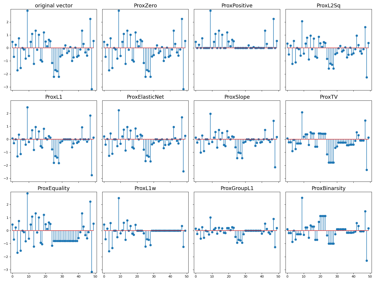
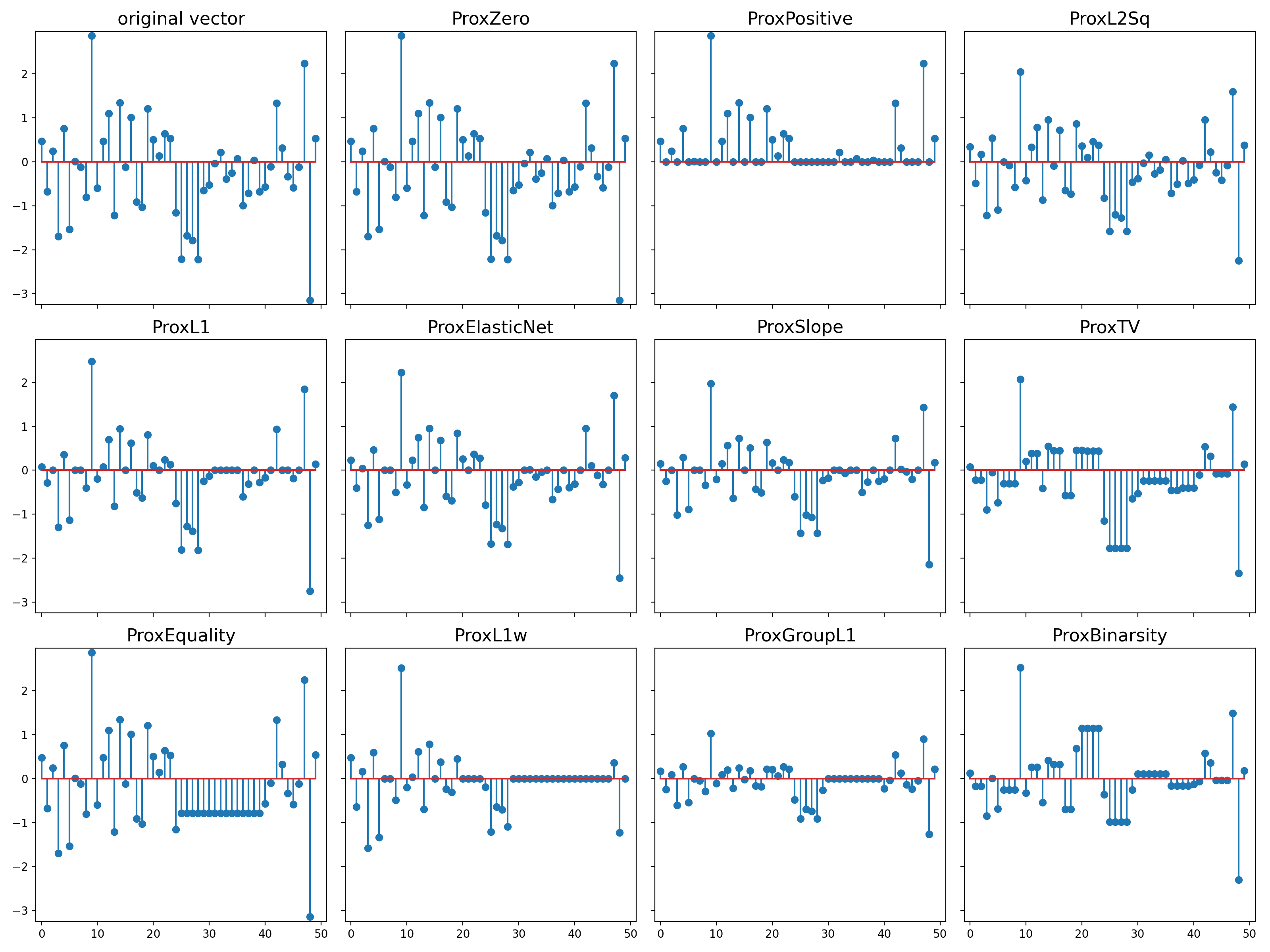
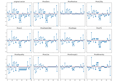
Here is an illustration of the effect of these proximal operators on an example.
"""
==============================
Examples of proximal operators
==============================

Plot examples of proximal operators available in tick
"""
import numpy as np
import matplotlib.pyplot as plt
from tick.prox import ProxL1, ProxElasticNet, ProxL2Sq, \
    ProxPositive, ProxSlope, ProxTV, ProxZero, ProxBinarsity, ProxGroupL1, \
    ProxEquality, ProxL1w

np.random.seed(12)
x = np.random.randn(50)
a, b = x.min() - 1e-1, x.max() + 1e-1
s = 0.4

proxs = [
    ProxZero(),
    ProxPositive(),
    ProxL2Sq(strength=s),
    ProxL1(strength=s),
    ProxElasticNet(strength=s, ratio=0.5),
    ProxSlope(strength=s),
    ProxTV(strength=s),
    ProxEquality(range=(25, 40)),
    ProxL1w(strength=s, weights=0.1 * np.arange(50, dtype=np.double)),
    ProxGroupL1(strength=2 * s, blocks_start=np.arange(0, 50, 10),
                blocks_length=10 * np.ones((5,))),
    ProxBinarsity(strength=s, blocks_start=np.arange(0, 50, 10),
                  blocks_length=10 * np.ones((5,)))
]

fig, _ = plt.subplots(3, 4, figsize=(16, 12), sharey=True, sharex=True)
fig.axes[0].stem(x)
fig.axes[0].set_title("original vector", fontsize=16)
fig.axes[0].set_xlim((-1, 51))
fig.axes[0].set_ylim((a, b))

for i, prox in enumerate(proxs):
    fig.axes[i + 1].stem(prox.call(x))
    fig.axes[i + 1].set_title(prox.name, fontsize=16)
    fig.axes[i + 1].set_xlim((-1, 51))
    fig.axes[i + 1].set_ylim((a, b))

plt.tight_layout()
plt.show()
(Source code, png, hires.png, pdf)
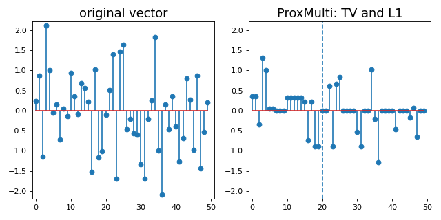
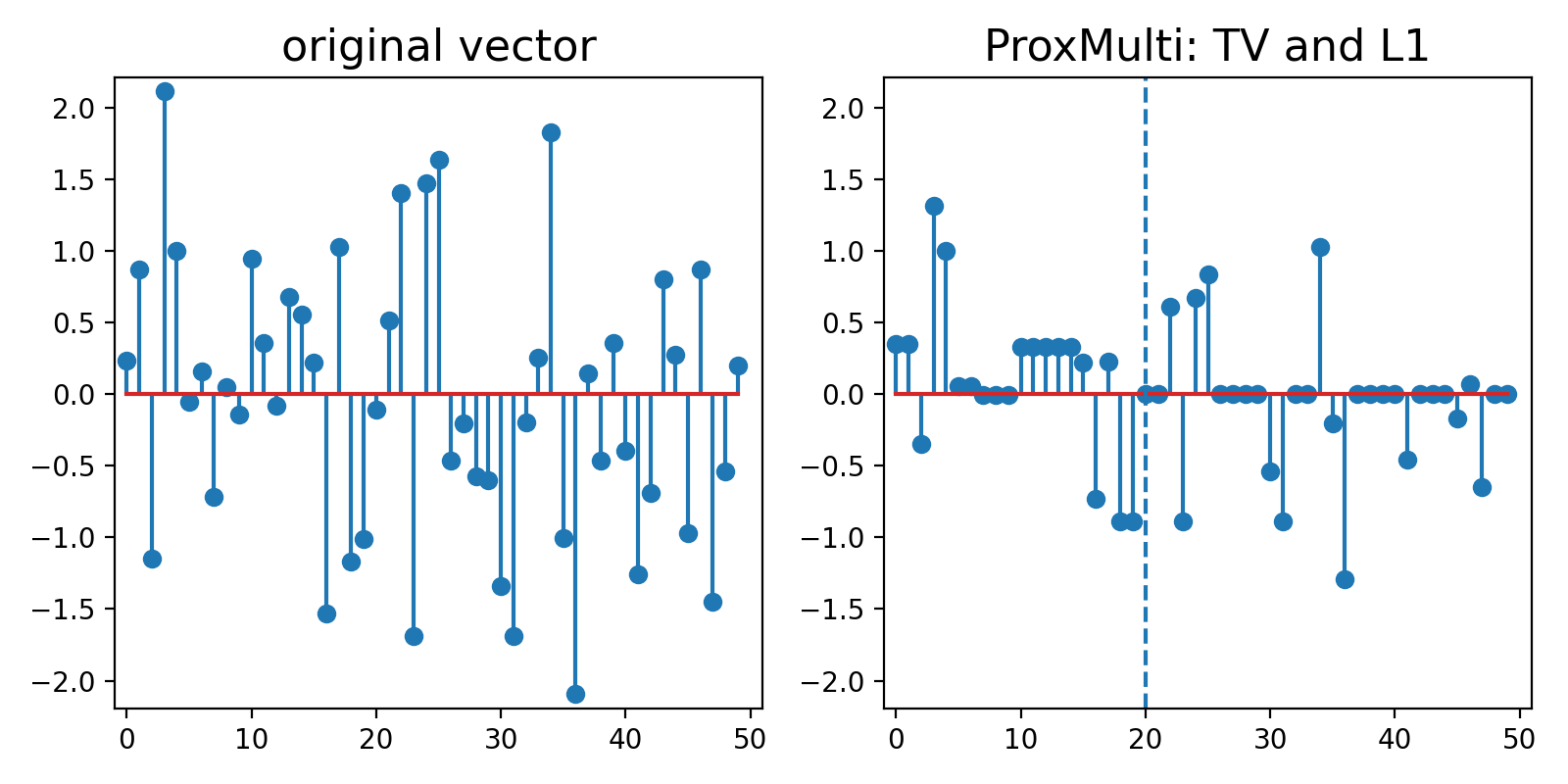
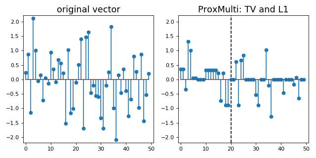
3. How to combine several prox ?
Another prox class is the ProxMulti that
allows to combine any proximal operators together.
It simply applies sequentially each operator passed to ProxMulti,
one after the other. Here is an example of combination of a total-variation penalization and L1 penalization
applied to different parts of a vector.
import numpy as np
import matplotlib.pyplot as plt
from tick.prox import ProxL1, ProxTV, ProxMulti

s = 0.4

prox = ProxMulti(
    proxs=(
        ProxTV(strength=s, range=(0, 20)),
        ProxL1(strength=2 * s, range=(20, 50))
    )
)

x = np.random.randn(50)
a, b = x.min() - 1e-1, x.max() + 1e-1

plt.figure(figsize=(8, 4))
plt.subplot(1, 2, 1)
plt.stem(x)
plt.title("original vector", fontsize=16)
plt.xlim((-1, 51))
plt.ylim((a, b))
plt.subplot(1, 2, 2)
plt.stem(prox.call(x))
plt.title("ProxMulti: TV and L1", fontsize=16)
plt.xlim((-1, 51))
plt.ylim((a, b))
plt.vlines(20, a, b, linestyles='dashed')
plt.tight_layout()
plt.show()
(Source code, png, hires.png, pdf)
4. The prox class API
Let us describe the prox API with the ProxL1
class, that provides the proximal operator of the function
\(g(w) = s \|w\|_1 = s \sum_{j=1}^d |w_j|\), where \(s\) corresponds
to the strength of penalization, and can be tuned using the strength
parameter.
import numpy as np
from tick.prox import ProxL1

prox = ProxL1(strength=1e-2)
print(prox)
prints
{
  "dtype": "float64",
  "name": "ProxL1",
  "positive": false,
  "range": null,
  "strength": 0.01
}
The positive parameter allows to enforce positivity, namely when positive=True then
the considered function is actually \(g(w) = s \|w\|_1 + \delta_{C}(x)\) where \(C\) is
the set of vectors with non-negative entries.
Note that no range was specified to this prox so that it is null (None) for now.
prox = ProxL1(strength=1e-2, range=(0, 30), positive=True)
print(prox)
prints
{
  "dtype": "float64",
  "name": "ProxL1",
  "positive": true,
  "range": [
    0,
    30
  ],
  "strength": 0.01
}
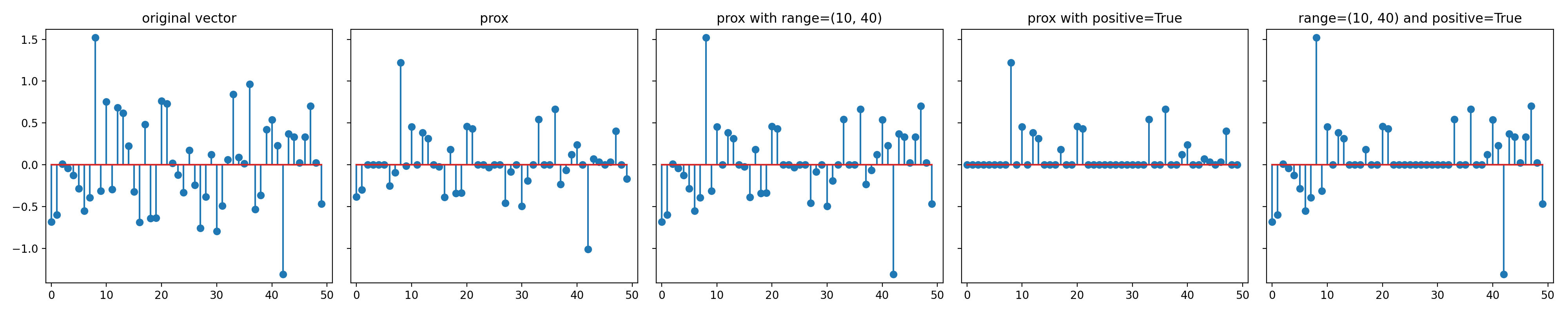
All prox classes provide a method call that computes \(\text{prox}_{g}(w, t)\)
where \(t\) is a parameter passed using the step argument.
The output of call can optionally be passed using the out argument (this
allows to avoid unnecessary copies, and thus extra memory allocation).
import numpy as np
import matplotlib.pyplot as plt
from tick.prox import ProxL1

x = 0.5 * np.random.randn(50)
a, b = x.min() - 1e-1, x.max() + 1e-1

proxs = [
    ProxL1(strength=0.),
    ProxL1(strength=3e-1),
    ProxL1(strength=3e-1, range=(10, 40)),
    ProxL1(strength=3e-1, positive=True),
    ProxL1(strength=3e-1, range=(10, 40), positive=True),
]

names = [
    "original vector",
    "prox",
    "prox with range=(10, 40)",
    "prox with positive=True",
    "range=(10, 40) and positive=True",
]

_, ax_list = plt.subplots(1, 5, figsize=(20, 4), sharey=True)

for prox, name, ax in zip(proxs, names, ax_list):
    ax.stem(prox.call(x))
    ax.set_title(name)
    ax.set_xlim((-1, 51))
    ax.set_ylim((a, b))

plt.tight_layout()
plt.show()
(Source code, png, hires.png, pdf)

The value of \(g\) is simply obtained using the value method
prox = ProxL1(strength=1., range=(5, 10))
val = prox.value(np.arange(10, dtype=np.double))
print(val)
simply prints
35.0
which corresponds to the sum of integers between 5 and 9 included.