tick.linear_model¶

1. Introduction¶

Given training data \((x_i, y_i) \in \mathbb R^d \times \mathbb R\) for \(i=1, \ldots, n\), tick considers, when solving a generalized linear model an objective of the form

where:

• \(w \in \mathbb R^d\) is a vector containing the model weights;

• \(b \in \mathbb R\) is the population intercept;

• \(\ell : \mathbb R^2 \rightarrow \mathbb R\) is a loss function

• \(g\) is a penalization function, see tick.prox for a list of available penalization technique

Depending on the model the label can be binary \(y_i \in \{ -1, 1 \}\) (binary classification), discrete \(y_i \in \mathbb N\) (Poisson models, see below) or continuous \(y_i \in \mathbb R\) (least-squares regression). The loss function \(\ell\) depends on the considered model, that are listed in 3. Models below. This modules proposes also end-user learner classes described below.

2. Learners¶

The following table lists the different learners that allows to train a model with several choices of penalizations and solvers.

These classes follow whenever possible the scikit-learn API, namely fit and predict methods, and follow the same naming conventions.

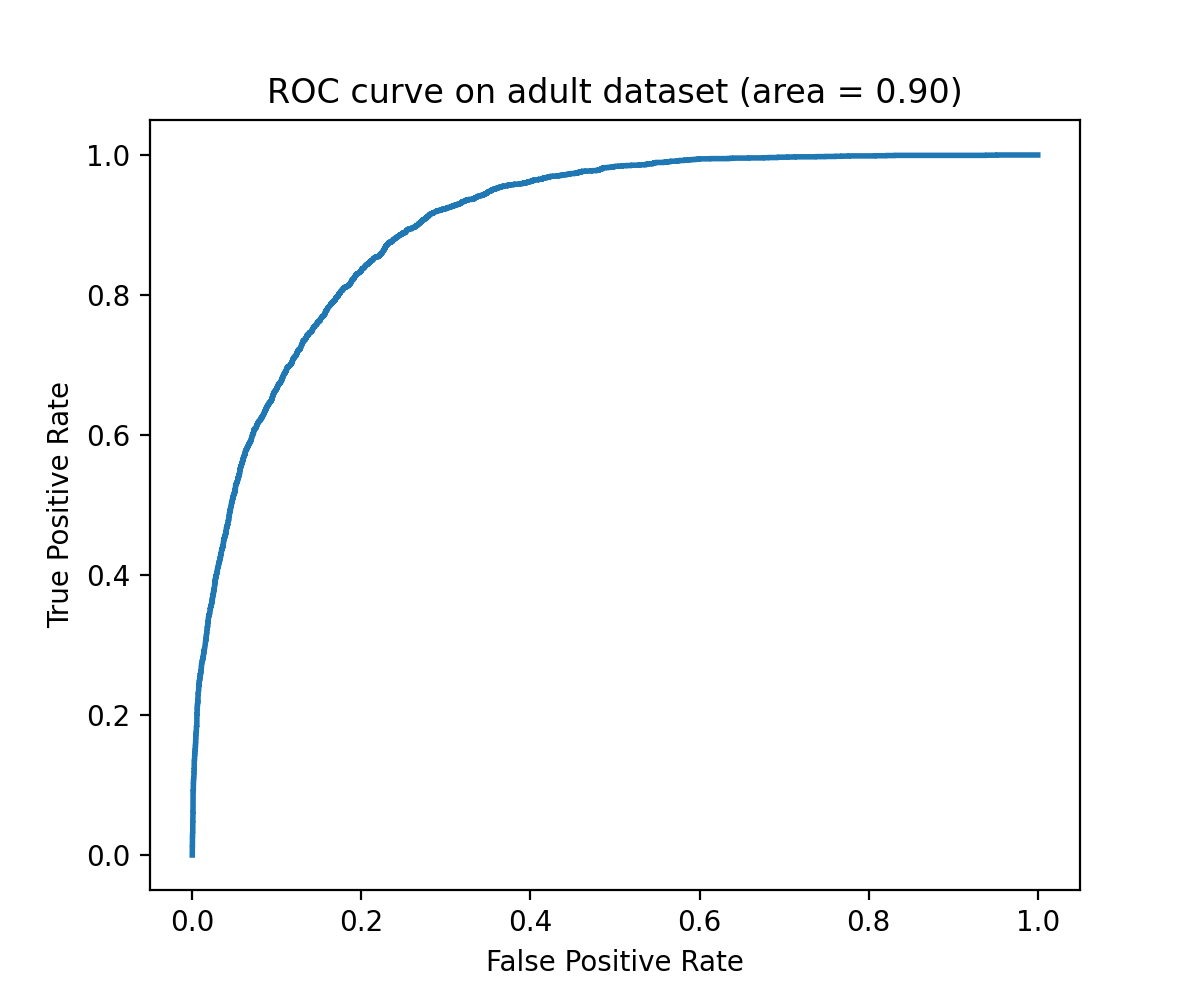
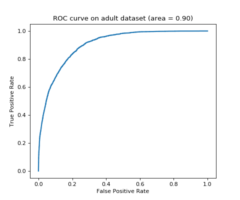
Example¶

"""
==============================================
Binary classification with logistic regression
==============================================

This code perform binary classification on adult dataset with logistic
regression learner (`tick.inference.LogisticRegression`).
"""

import matplotlib.pyplot as plt
from sklearn.metrics import roc_curve, auc

from tick.linear_model import LogisticRegression
from tick.dataset import fetch_tick_dataset

train_set = fetch_tick_dataset('binary/adult/adult.trn.bz2')
test_set = fetch_tick_dataset('binary/adult/adult.tst.bz2')

learner = LogisticRegression()
learner.fit(train_set[0], train_set[1])

predictions = learner.predict_proba(test_set[0])
fpr, tpr, _ = roc_curve(test_set[1], predictions[:, 1])

plt.figure(figsize=(6, 5))
plt.plot(fpr, tpr, lw=2)
plt.title("ROC curve on adult dataset (area = {:.2f})".format(auc(fpr, tpr)))
plt.ylabel("True Positive Rate")
plt.xlabel("False Positive Rate")

plt.show()

(Source code, png, hires.png, pdf)

3. Models¶

In tick a model class gives information about a statistical model. Depending on the case, it gives first order information (loss, gradient) or second order information (hessian norm evaluation). In this module, a model corresponds to the choice of a loss function, that are described below. The advantages of using one or another loss are explained in the documentation of the classes themselves. The following table lists the different losses implemented for now in this module, its associated class and label type.

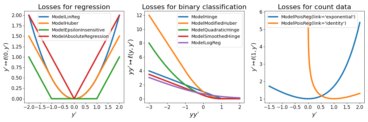
3.1. Description of the available models¶

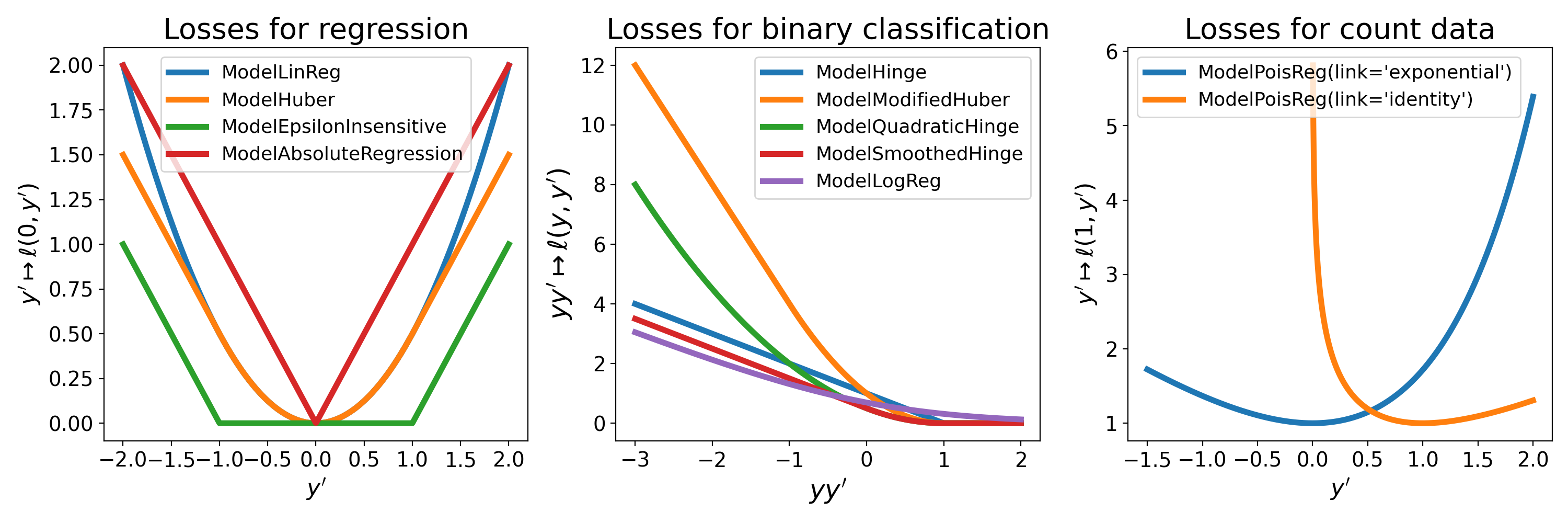
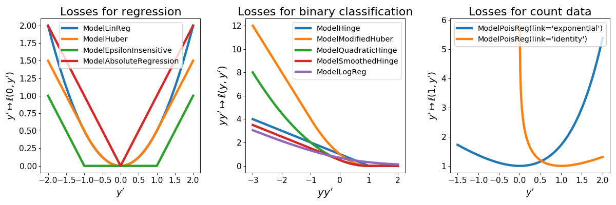
On the following graph we represent the different losses available in tick for supervised linear learning. Note that ModelHuber, ModelEpsilonInsensitive, ModelModifiedHuber and ModelAbsoluteRegression are available through the tick.robust module.

(Source code, png, hires.png, pdf)

ModelLinReg¶

This is least-squares regression with loss

\[\ell(y, y') = \frac 12 (y - y')^2\]

for \(y, y' \in \mathbb R\)

---

ModelLogReg¶

Logistic regression for binary classification with loss

\[\ell(y, y') = \log(1 + \exp(-y y'))\]

for \(y \in \{ -1, 1\}\) and \(y' \in \mathbb R\)

---

ModelHinge¶

This is the hinge loss for binary classification given by

\[\begin{split}\ell(y, y') = \begin{cases} 1 - y y' &\text{ if } y y' < 1 \\ 0 &\text{ if } y y' \geq 1 \end{cases}\end{split}\]

for \(y \in \{ -1, 1\}\) and \(y' \in \mathbb R\)

---

ModelQuadraticHinge¶

This is the quadratic hinge loss for binary classification given by

\[\begin{split}\ell(y, y') = \begin{cases} \frac 12 (1 - y y')^2 &\text{ if } y y' < 1 \\ 0 &\text{ if } y y' \geq 1 \end{cases}\end{split}\]

for \(y \in \{ -1, 1\}\) and \(y' \in \mathbb R\)

---

ModelSmoothedHinge¶

This is the smoothed hinge loss for binary classification given by

\[\begin{split}\ell(y, y') = \begin{cases} 1 - y y' - \frac \delta 2 &\text{ if } y y' \leq 1 - \delta \\ \frac{(1 - y y')^2}{2 \delta} &\text{ if } 1 - \delta < y y' < 1 \\ 0 &\text{ if } y y' \geq 1 \end{cases}\end{split}\]

for \(y \in \{ -1, 1\}\) and \(y' \in \mathbb R\), where \(\delta \in (0, 1)\) can be tuned using the smoothness parameter. Note that \(\delta = 0\) corresponds to the hinge loss.

---

ModelPoisReg¶

Poisson regression with exponential link with loss corresponds to the loss

\[\ell(y, y') = e^{y'} - y y'\]

for \(y \in \mathbb N\) and \(y' \in \mathbb R\) and is obtained using link='exponential'. Poisson regression with identity link, namely with loss

\[\ell(y, y') = y' - y \log(y')\]

for \(y \in \mathbb N\) and \(y' > 0\) is obtained using link='identity'.

3.2. The model class API¶

All model classes allow to compute the loss (value of the objective function \(f\)) and its gradient. Let us illustrate this with the logistic regression model. First, we need to simulate data.

import numpy as np
from tick.linear_model import SimuLogReg
from tick.simulation import weights_sparse_gauss

n_samples, n_features = 2000, 50
weights0 = weights_sparse_gauss(n_weights=n_features, nnz=10)
intercept0 = 1.
X, y = SimuLogReg(weights0, intercept=intercept0, seed=123,
                  n_samples=n_samples, verbose=False).simulate()

Now, we can create the model object for logistic regression

import numpy as np
from tick.linear_model import ModelLogReg

model = ModelLogReg(fit_intercept=True).fit(X, y)
print(model)

outputs

{
  "dtype": "float64",
  "fit_intercept": true,
  "n_calls_grad": 0,
  "n_calls_loss": 0,
  "n_calls_loss_and_grad": 0,
  "n_coeffs": 51,
  "n_features": 50,
  "n_passes_over_data": 0,
  "n_samples": 2000,
  "n_threads": 1,
  "name": "ModelLogReg"
}

Printing any object in tick returns a json formatted description of it. We see that this model uses 50 features, 51 coefficients (including the intercept), and that it received 2000 sample points. Now we can compute the loss of the model using the loss method (its objective, namely the value of the function \(f\) to be minimized) by using

coeffs0 = np.concatenate([weights0, [intercept0]])
print(model.loss(coeffs0))

which outputs

0.3551082120992899

while

print(model.loss(np.ones(model.n_coeffs)))

outputs

5.793300908869233

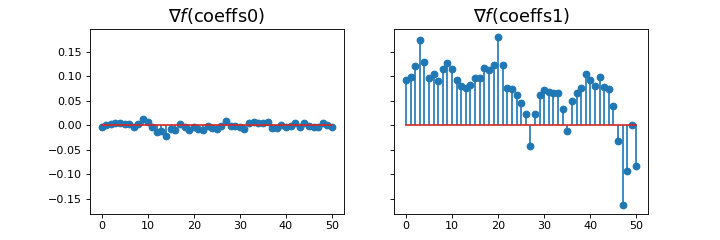
which is explained by the fact that the loss is larger for a parameter which is far from the ones used for the simulation. The gradient of the model can be computed using the grad method

_, ax = plt.subplots(1, 2, sharey=True, figsize=(9, 3))
ax[0].stem(model.grad(coeffs0))
ax[0].set_title(r"$\nabla f(\mathrm{coeffs0})$", fontsize=16)
ax[1].stem(model.grad(np.ones(model.n_coeffs)))
ax[1].set_title(r"$\nabla f(\mathrm{coeffs1})$", fontsize=16)

which plots

(Source code, png, hires.png, pdf)

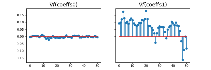
We observe that the gradient near the optimum is much smaller than far from it. Model classes can be used with any solver class, by simply passing them through the solver’s set_model method, see tick.solver.

What’s under the hood?

All model classes have a loss and grad method, that are used by batch algorithms to fit the model. These classes contains a C++ object, that does the computations. Some methods are hidden within this C++ object, and are accessible only through C++ (such as loss_i and grad_i that compute the gradient using the single data point \((x_i, y_i)\)). These hidden methods are used in the stochastic solvers, and are available through C++ only for efficiency.

4. Simulation¶

Simulation of several linear models can be done using the following classes. All simulation classes simulates a features matrix \(\boldsymbol X\) with rows \(x_i\) and a labels vector \(y\) with coordinates \(y_i\) for \(i=1, \ldots, n\), that are i.i.d realizations of a random vector \(X\) and a scalar random variable \(Y\). The conditional distribution of \(Y | X\) is \(\mathbb P(Y=y | X=x)\), where \(\mathbb P\) depends on the considered model.

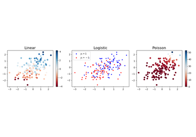
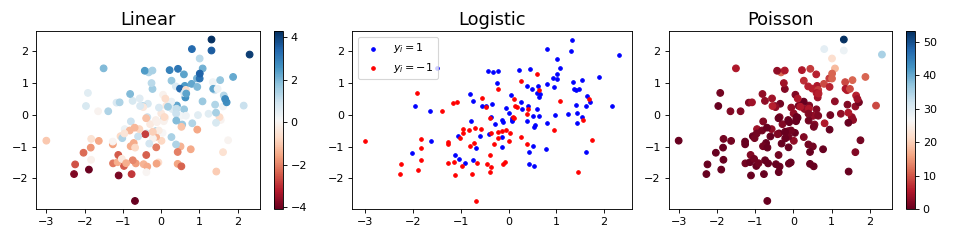
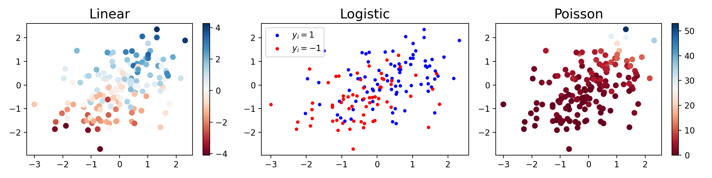
Example

"""
=============================
Linear models data simulation
=============================

Generates Linear, Logistic and Poisson regression realizations given a 
weight vector.
"""

import matplotlib.pyplot as plt
import numpy as np
from tick.linear_model import SimuLinReg, SimuLogReg, SimuPoisReg

n_samples, n_features = 150, 2

weights0 = np.array([0.3, 1.2])
intercept0 = 0.5

simu_linreg = SimuLinReg(weights0, intercept0, n_samples=n_samples, seed=123,
                         verbose=False)
X_linreg, y_linreg = simu_linreg.simulate()

simu_logreg = SimuLogReg(weights0, intercept0, n_samples=n_samples, seed=123,
                         verbose=False)
X_logreg, y_logreg = simu_logreg.simulate()

simu_poisreg = SimuPoisReg(weights0, intercept0, n_samples=n_samples,
                           link='exponential', seed=123, verbose=False)
X_poisreg, y_poisreg = simu_poisreg.simulate()

plt.figure(figsize=(12, 3))

plt.subplot(1, 3, 1)
plt.scatter(*X_linreg.T, c=y_linreg, cmap='RdBu')
plt.colorbar()
plt.title('Linear', fontsize=16)

plt.subplot(1, 3, 2)
plt.scatter(*X_logreg[y_logreg == 1].T, color='b', s=10, label=r'$y_i=1$')
plt.scatter(*X_logreg[y_logreg == -1].T, color='r', s=10, label=r'$y_i=-1$')
plt.legend(loc='upper left')
plt.title('Logistic', fontsize=16)

plt.subplot(1, 3, 3)
plt.scatter(*X_poisreg.T, c=y_poisreg, cmap='RdBu')
plt.colorbar()
plt.title('Poisson', fontsize=16)

plt.tight_layout()
plt.show()

(Source code, png, hires.png, pdf)