tick.robust
This module provides tools for robust inference of generalized linear models and outliers detection. It proposes two set of things: a learner for least-squares regression with individual intercepts, see 1. Regression with individual intercepts and a set of losses for robust supervised learning, see 2. Robust losses.
1. Regression with individual intercepts
In this section, we describe the approach used in the
RobustLinearRegression learner.
It allows to detect outliers and to fit a least-squares regression
model at the same time. Namely, given training data
\((x_i, y_i) \in \mathbb R^d \times \mathbb R\) for \(i=1, \ldots, n\),
it considers the following problem
where \(|w_{(j)}|\) is decreasing, \(w \in \mathbb R^d\) is a vector containing the model weights, \(\mu = [\mu_1 \cdots \mu_n] \in \mathbb R^n\) is a vector containing individual intercepts, \(b \in \mathbb R\) is the population intercept, \(\ell : \mathbb R^2 \rightarrow \mathbb R\) is the least-squares loss and \(g\) is a penalization function for the model weights, for which different choices are possible, see tick.prox. Note that in this problem the vector of individual intercepts \(\mu\) is penalized by a sorted-L1 norm, also called SLOPE, see tick.prox for details, where the weights are given by
where \(\alpha\) stands for the FDR level for the support detection of
\(\mu\), that can be tuned with the fdr parameter.
The global penalization level \(s\) corresponds to
the inverse of the C_sample_intercepts parameter.
|
Robust linear regression learner. |
Tools for robust estimation of the standard-deviation
Some tools for the robust estimation of the standard deviation are also provided.
|
Robust estimation of the standard deviation, based on the Corrected Median Absolute Deviation (MAD) of x. |
|
Robust estimation of the standard deviation, based on the inter-quartile (IQR) distance of x. |
Example
"""
===========================
Robust linear model example
===========================

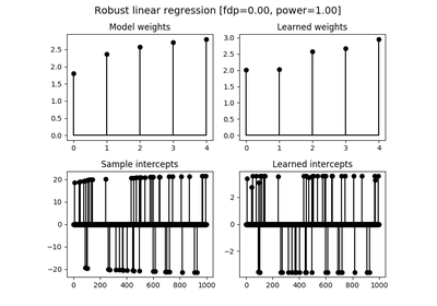
In this example with simulate a linear regression model with 1000 samples and
5 features. The simulated data is contaminated by 20% of outliers, in the form
of sparse sample intercepts (thus only on 20% of samples).

We illustrate the estimated linear regression weights and sample intercepts
obtained by the ``RobustLinearRegression`` learner, where we also compute the
false discovery proportion and power of the method for the multi-test problem of
outliers detection.
Note that the penalization level ``C_sample_intercepts`` of the sample
intercepts should be chosen as n_samples / noise_level, where noise_level is
obtained by a robust estimation of the noise's standard deviation.
We simply use here the `tick.inference.std_iqr` estimator.

Note that we don't use penalization on the model weights here, while other
penalizations are available, by changing the ``penalty`` parameter and by
giving a ``C`` value for the level of penalization.
Default is ``penalty='l2'``, namely ridge penalization, while ``penalty='l1'``
or ``penalty='slope'`` can be used when the number of features is large.
"""
import numpy as np
from matplotlib import pyplot as plt
from tick.simulation import weights_sparse_gauss, \
    features_normal_cov_toeplitz
from tick.robust import RobustLinearRegression, std_iqr
from tick.metrics import support_fdp, support_recall

np.random.seed(1)

n_samples = 1000
n_features = 5
noise_level = 1.
n_outliers = 50
outliers_intensity = 5.

intercept0 = -3.
log_linspace = np.log(n_features * np.linspace(1, 10, n_features))
weights0 = np.sqrt(2 * log_linspace)

sample_intercepts0 = weights_sparse_gauss(n_weights=n_samples, nnz=n_outliers)
idx_nnz = sample_intercepts0 != 0
log_linspace = np.log(n_samples * np.linspace(1, 10, n_outliers))
sample_intercepts0[idx_nnz] = outliers_intensity * np.sqrt(2 * log_linspace) \
    * np.sign(sample_intercepts0[idx_nnz])

X = features_normal_cov_toeplitz(n_samples, n_features, 0.5)

y = X.dot(weights0) + noise_level * np.random.randn(n_samples) \
    + intercept0 + sample_intercepts0

target_fdr = 0.1
noise_level = std_iqr(y)
learner = RobustLinearRegression(
    C_sample_intercepts=2 * n_samples / noise_level, penalty='none',
    fdr=target_fdr, verbose=False)
learner.fit(X, y)

fdp_ = support_fdp(sample_intercepts0, learner.sample_intercepts)
power_ = support_recall(sample_intercepts0, learner.sample_intercepts)

fig = plt.figure(figsize=(7, 6))
titles = [
    'Model weights', 'Learned weights', 'Sample intercepts',
    'Learned intercepts'
]
vectors = [
    weights0, learner.weights, sample_intercepts0, learner.sample_intercepts
]
for idx_plot, title, vector in zip(range(221, 225), titles, vectors):
    ax = fig.add_subplot(idx_plot)
    ax.stem(vector)
    ax.set_title(title, fontsize=12)
fig.suptitle(
    'Robust linear regression [fdp=%.2f, power=%.2f]' % (fdp_, power_),
    fontsize=14)
fig.tight_layout(rect=[0, 0.03, 1, 0.95])
plt.show()
(Source code, png, hires.png, pdf)

2. Robust losses
Tick also provides losses for robust inference when it is believed that data contains
outliers. It also provides the model
ModelLinRegWithIntercepts which is
used in the RobustLinearRegression
described above.
Model |
Type |
Label type |
Class |
|---|---|---|---|
Linear regression with intercepts |
Regression |
Continuous |
|
Huber regression |
Regression |
Continuous |
|
Epsilon-insensitive regression |
Regression |
Continuous |
|
Absolute regression |
Regression |
Continuous |
|
Modified Huber loss |
Classification |
Binary |
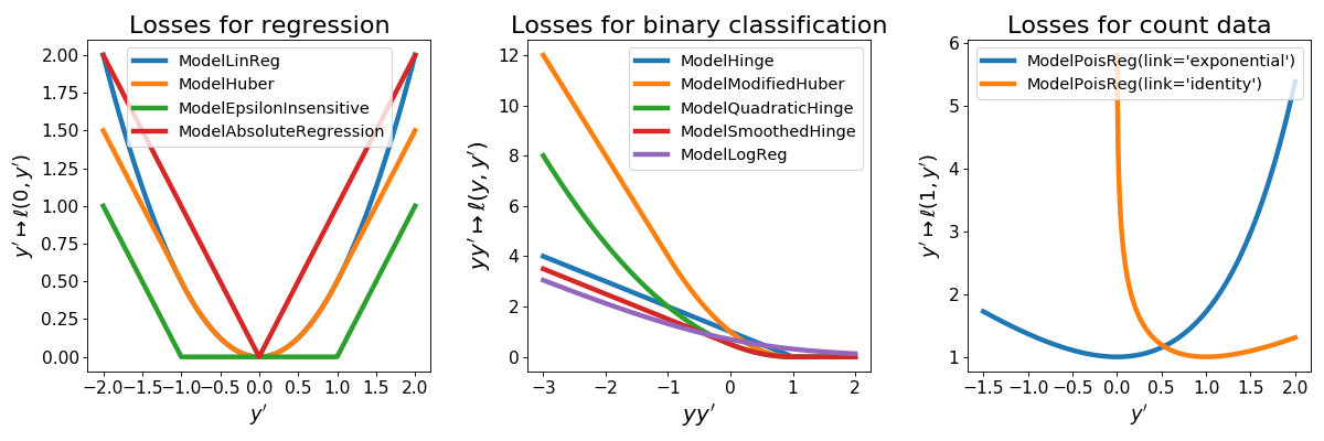
The robust losses are illustrated in the following picture, among the other losses provided in the tick.linear_model module.
(Source code, png, hires.png, pdf)

ModelHuber
The Huber loss for robust regression (less sensitive to outliers) is given by
for \(y, y' \in \mathbb R\), where \(\delta > 0\) can be tuned
using the threshold argument.
ModelEpsilonInsensitive
Epsilon-insensitive loss, given by
for \(y, y' \in \mathbb R\), where \(\epsilon > 0\) can be tuned using
the threshold argument.
ModelAbsoluteRegression
The L1 loss given by
for \(y, y' \in \mathbb R\)
ModelModifiedHuber
The modified Huber loss, used for robust classification (less sensitive to outliers). The loss is given by
for \(y \in \{ -1, 1\}\) and \(y' \in \mathbb R\)