tick.plot
This module gathers all the plotting utilities of tick, namely plots for a
solver’s history, see 1. History plot, plots for Hawkes processes, see 2. Plots for Hawkes processes,
plots for point process simulations 3. Plots for point process simulation and some other useful plots, see
4. Miscellaneous plots.
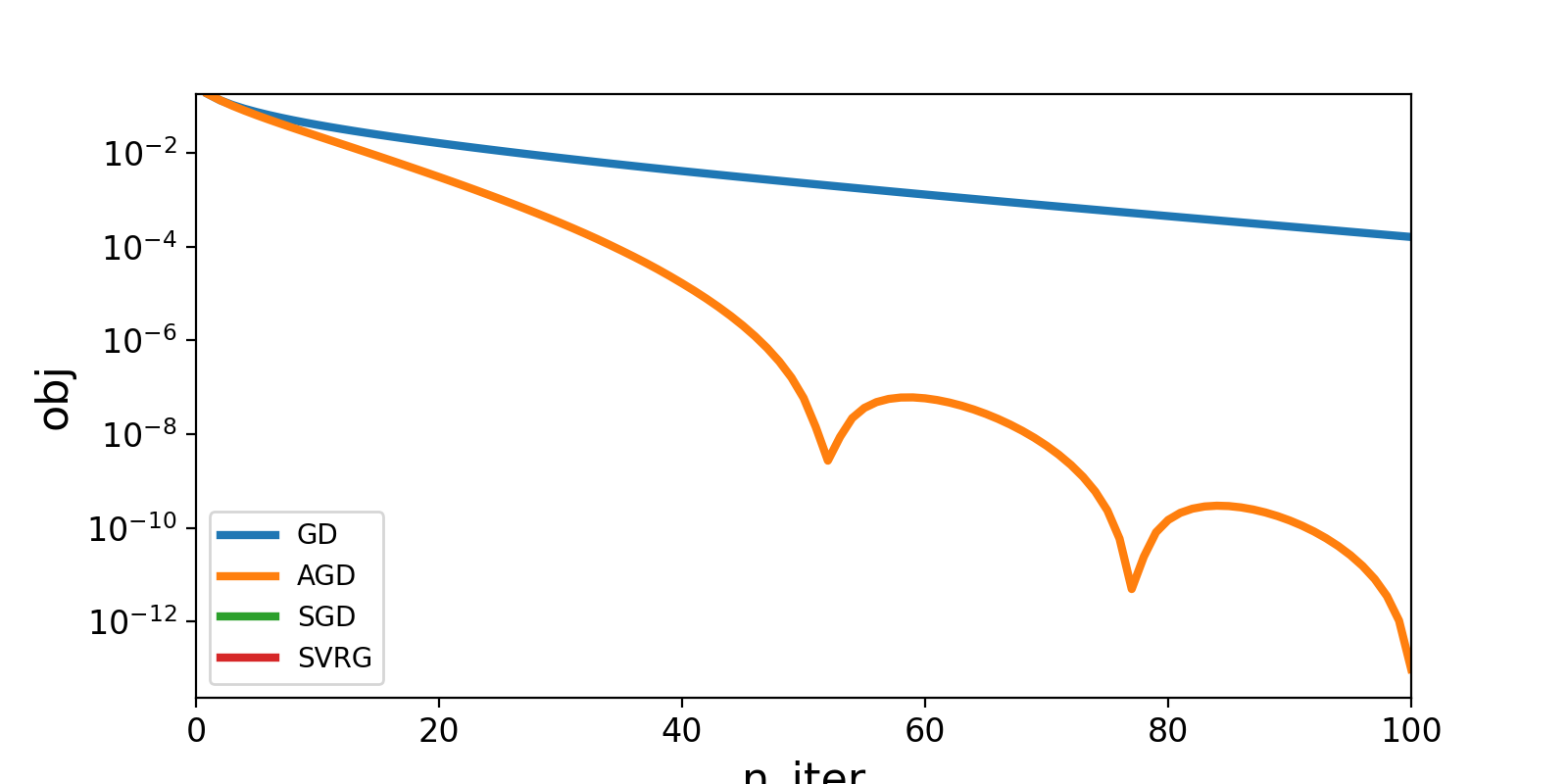
1. History plot
This plot is used to compare the efficiency of optimization algorithms
implemented in tick.solver.
|
Plot the history of convergence of learners or solvers. |
Example
import numpy as np
from tick.linear_model import ModelLogReg ,SimuLogReg
from tick.simulation import weights_sparse_gauss
from tick.solver import GD, AGD, SGD, SVRG, SDCA
from tick.prox import ProxElasticNet, ProxL1
from tick.plot import plot_history

n_samples, n_features, = 5000, 50
weights0 = weights_sparse_gauss(n_features, nnz=10)
intercept0 = 0.2
X, y = SimuLogReg(weights=weights0, intercept=intercept0,
                  n_samples=n_samples, seed=123, verbose=False).simulate()

model = ModelLogReg(fit_intercept=True).fit(X, y)
prox = ProxElasticNet(strength=1e-3, ratio=0.5, range=(0, n_features))

solver_params = {'max_iter': 100, 'tol': 0., 'verbose': False}
x0 = np.zeros(model.n_coeffs)

gd = GD(linesearch=False, **solver_params).set_model(model).set_prox(prox)
gd.solve(x0, step=1 / model.get_lip_best())

agd = AGD(linesearch=False, **solver_params).set_model(model).set_prox(prox)
agd.solve(x0, step=1 / model.get_lip_best())

sgd = SGD(**solver_params).set_model(model).set_prox(prox)
sgd.solve(x0, step=500.)

svrg = SVRG(**solver_params).set_model(model).set_prox(prox)
svrg.solve(x0, step=1 / model.get_lip_max())

plot_history([gd, agd, sgd, svrg], log_scale=True, dist_min=True)
(Source code, png, hires.png, pdf)

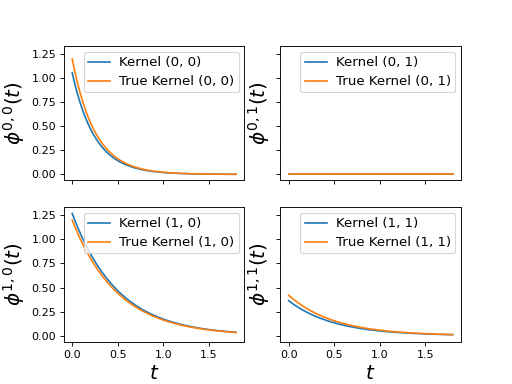
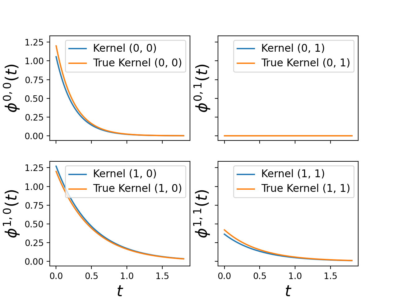
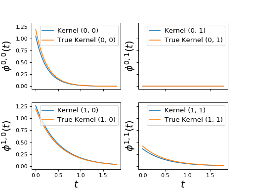
2. Plots for Hawkes processes
These plots are used to observe hawkes parameters obtained by hawkes learners.
|
Generic function to plot Hawkes kernels. |
|
Generic function to plot Hawkes kernel norms. |
|
Function used to plot basis of kernels |
Example
from tick.plot import plot_hawkes_kernels
from tick.hawkes import SimuHawkesExpKernels, SimuHawkesMulti, HawkesExpKern
import matplotlib.pyplot as plt

end_time = 1000
n_realizations = 10

decays = [[4., 1.], [2., 2.]]
baseline = [0.12, 0.07]
adjacency = [[.3, 0.], [.6, .21]]

hawkes_exp_kernels = SimuHawkesExpKernels(
    adjacency=adjacency, decays=decays, baseline=baseline,
    end_time=end_time, verbose=False, seed=1039)

multi = SimuHawkesMulti(hawkes_exp_kernels, n_simulations=n_realizations)

multi.end_time = [(i + 1) / 10 * end_time for i in range(n_realizations)]
multi.simulate()

learner = HawkesExpKern(decays, penalty='l1', C=10)
learner.fit(multi.timestamps)

plot_hawkes_kernels(learner, hawkes=hawkes_exp_kernels)
(Source code, png, hires.png, pdf)
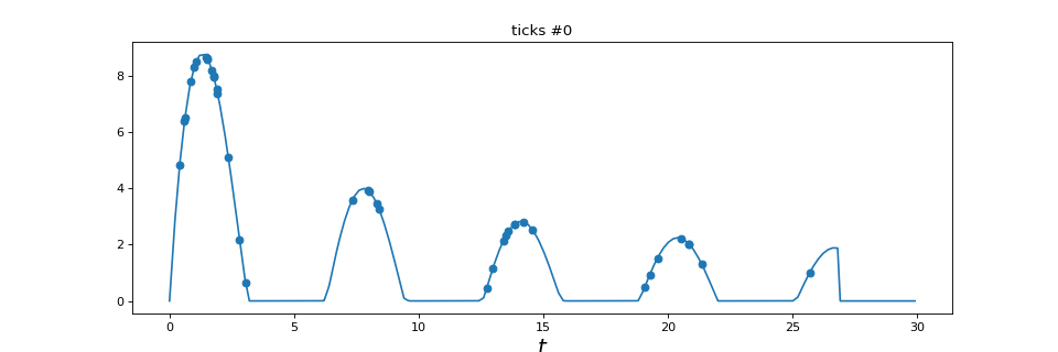
3. Plots for point process simulation
This plot is used to plot a point process simulation.
|
Plot point process realization |
Example
"""
========================================
Inhomogeneous Poisson process simulation
========================================

This example show how to simulate any inhomogeneous Poisson process. Its
intensity is modeled through `tick.base.TimeFunction`
"""

import numpy as np
from tick.base import TimeFunction

from tick.plot import plot_point_process
from tick.hawkes import SimuInhomogeneousPoisson

run_time = 30

T = np.arange((run_time * 0.9) * 5, dtype=float) / 5
Y = np.maximum(
    15 * np.sin(T) * (np.divide(np.ones_like(T),
                                np.sqrt(T + 1) + 0.1 * T)), 0.001)

tf = TimeFunction((T, Y), dt=0.01)

# We define a 1 dimensional inhomogeneous Poisson process with the
# intensity function seen above
in_poi = SimuInhomogeneousPoisson([tf], end_time=run_time, verbose=False)

# We activate intensity tracking and launch simulation
in_poi.track_intensity(0.1)
in_poi.simulate()

# We plot the resulting inhomogeneous Poisson process with its
# intensity and its ticks over time
plot_point_process(in_poi)
(Source code, png, hires.png, pdf)
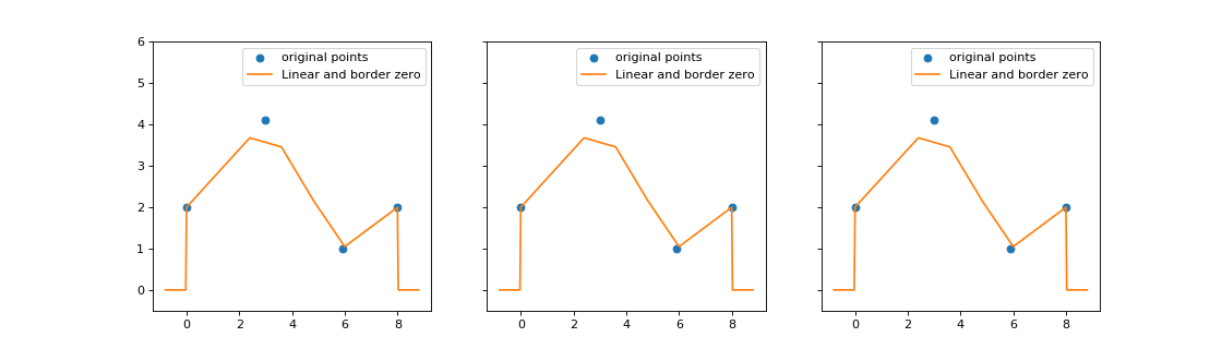
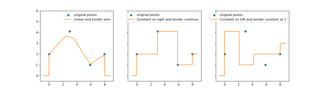
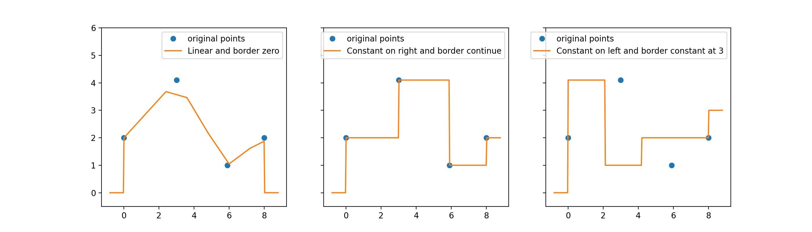
4. Miscellaneous plots
Some other plots are particularly useful: plots for TimeFunction <tick.base.TimeFunction>`
and a plot generating several stem plots at the same time, allowing matplotlib
or bokeh rendering.
|
Quick plot of a |
|
Plot several stem plots using either matplotlib or bokeh rendering. |
Example
import matplotlib.pyplot as plt
import numpy as np
from tick.base import TimeFunction
from tick.plot import plot_timefunction

T = np.array([0, 3, 5.9, 8.001], dtype=float)
Y = np.array([2, 4.1, 1, 2], dtype=float)

tf_1 = TimeFunction((T, Y), dt=1.2)
tf_2 = TimeFunction((T, Y), border_type=TimeFunction.BorderContinue,
                    inter_mode=TimeFunction.InterConstRight, dt=0.01)
tf_3 = TimeFunction((T, Y), border_type=TimeFunction.BorderConstant,
                    inter_mode=TimeFunction.InterConstLeft, border_value=3)

time_functions = [tf_1, tf_2, tf_3]

_, ax_list = plt.subplots(1, 3, figsize=(14, 4), sharey=True)

for tf, ax in zip(time_functions, ax_list):
    plot_timefunction(tf, ax=ax)
    ax.set_ylim([-0.5, 6.0])
plt.show()
(Source code, png, hires.png, pdf)