tick.plot.plot_history
- tick.plot.plot_history(solvers, x='n_iter', y='obj', labels=None, show=True, log_scale: bool = False, dist_min: bool = False, rendering: str = 'matplotlib', ax=None)[source]
Plot the history of convergence of learners or solvers.
It is used to compare easily their convergence performance.
- Parameters:
solvers :
listofobjectwith and history to plot, namely solvers(children of
tick.solver.base.Solver) or learners (children oftick.hawkes.inference.base.LearnerOptim)x :
str, default=’n_iter’if ‘n_iter’ : iteration number
if ‘time’ : computation time
y :
str, default=’obj’- if ‘obj’the objective (value of the function minimized).
Other choices are possible, any of those present in the history
labels :
listofstr, default=NoneLabel of each solver in the legend. If set to None then the class name of each solver will be used.
show :
bool, default=`True`if
True, show the plot. Otherwise an explicit call to the show function is necessary. Useful when superposing several plots.log_scale :
bool, default=`False`If
True, then y-axis is on a log-scaledist_min :
bool, default=`False`If
True, plot the difference betweenyof each solver and the minimalyof all solvers. This is useful when comparing solvers on a logarithmic scale, to illustrate linear convergence of algorithmsrendering : {‘matplotlib’, ‘bokeh’}, default=’matplotlib’
Rendering library. ‘bokeh’ might fail if the module is not installed.
ax :
listofmatplotlib.axes, default=NoneIf not None, the figure will be plot on this axis and show will be set to False. Used only with matplotlib