Automatic step choice
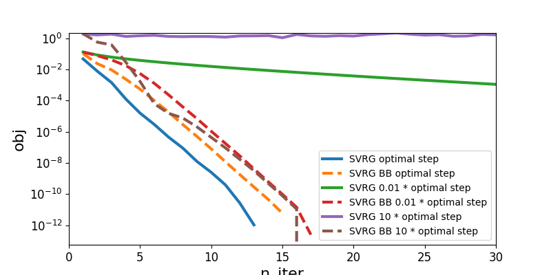
This example presents automatic step choice for SVRG thanks to Barzilai Borwein algorithm. This allows SVRG to be way less sensitive to the choice of the step. In this example we use a toy problem for which we know the theoretical optimal step and presents how SVRG deals with badly chosen steps.
Tan, C., Ma, S., Dai, Y. H., & Qian, Y. (2016). Barzilai-Borwein step size for stochastic gradient descent. In Advances in Neural Information Processing Systems.
Python source code: plot_svrg_with_auto_step.py
import numpy as np
import matplotlib.pyplot as plt
from cycler import cycler

from tick.simulation import weights_sparse_gauss
from tick.solver import SVRG
from tick.linear_model import SimuLogReg, ModelLogReg
from tick.prox import ProxElasticNet
from tick.plot import plot_history

n_samples, n_features, = 5000, 50
weights0 = weights_sparse_gauss(n_features, nnz=10)
intercept0 = 0.2
X, y = SimuLogReg(weights=weights0, intercept=intercept0, n_samples=n_samples,
                  seed=123, verbose=False).simulate()

model = ModelLogReg(fit_intercept=True).fit(X, y)
prox = ProxElasticNet(strength=1e-3, ratio=0.5, range=(0, n_features))
x0 = np.zeros(model.n_coeffs)

optimal_step = 1 / model.get_lip_max()
tested_steps = [optimal_step, 1e-2 * optimal_step, 10 * optimal_step]

solvers = []
solver_labels = []

for step in tested_steps:
    svrg = SVRG(max_iter=30, tol=1e-10, verbose=False)
    svrg.set_model(model).set_prox(prox)
    svrg.solve(step=step)

    svrg_bb = SVRG(max_iter=30, tol=1e-10, verbose=False, step_type='bb')
    svrg_bb.set_model(model).set_prox(prox)
    svrg_bb.solve(step=step)

    solvers += [svrg, svrg_bb]

    optimal_factor = step / optimal_step
    if optimal_factor != 1:
        solver_labels += [
            'SVRG {:.2g} * optimal step'.format(optimal_factor),
            'SVRG BB {:.2g} * optimal step'.format(optimal_factor)
        ]
    else:
        solver_labels += [
            'SVRG optimal step'.format(optimal_factor),
            'SVRG BB optimal step'.format(optimal_factor)
        ]

# To easily differentiate fixed steps from Barzilai Borwein steps SVRG solvers
plt.rc('axes', prop_cycle=(cycler('linestyle', ['-', '--'])))
plot_history(solvers=solvers, labels=solver_labels, log_scale=True,
             dist_min=True)
Total running time of the example: 0.56 seconds ( 0 minutes 0.56 seconds)