tick.solver.SVRG¶

class tick.solver.SVRG(step: float = None, epoch_size: int = None, rand_type: str = 'unif', tol: float = 1e-10, max_iter: int = 10, verbose: bool = True, print_every: int = 1, record_every: int = 1, seed: int = -1, variance_reduction: str = 'last', step_type: str = 'fixed', n_threads: int = 1)[source]¶

Stochastic Variance Reduced Gradient solver

For the minimization of objectives of the form

\[\frac 1n \sum_{i=1}^n f_i(w) + g(w),\]

where the functions \(f_i\) have smooth gradients and \(g\) is prox-capable. Function \(f = \frac 1n \sum_{i=1}^n f_i\) corresponds to the model.loss method of the model (passed with set_model to the solver) and \(g\) corresponds to the prox.value method of the prox (passed with the set_prox method). One iteration of SVRG corresponds to the following iteration applied epoch_size times:

\[w \gets \mathrm{prox}_{\eta g} \big(w - \eta (\nabla f_i(w) - \nabla f_i(\bar{w}) + \nabla f(\bar{w}) \big),\]

where \(i\) is sampled at random (strategy depends on rand_type) at each iteration, and where \(\bar w\) and \(\nabla f(\bar w)\) are updated at the beginning of each epoch, with a strategy that depend on the variance_reduction parameter. The step-size \(\eta\) can be tuned with step, the seed of the random number generator for generation of samples \(i\) can be seeded with seed. The iterations stop whenever tolerance tol is achieved, or after max_iter epochs (namely max_iter \(\times\) epoch_size iterates). The obtained solution \(w\) is returned by the solve method, and is also stored in the solution attribute of the solver.

Internally, SVRG has dedicated code when the model is a generalized linear model with sparse features, and a separable proximal operator: in this case, each iteration works only in the set of non-zero features, leading to much faster iterates.

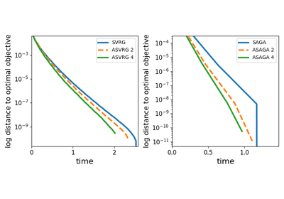
Moreover, when n_threads > 1, this class actually implements parallel and asynchronous updates of \(w\), which is likely to accelerate optimization, depending on the sparsity of the dataset, and the number of available cores.

Parameters:

step : float

Step-size parameter, the most important parameter of the solver. Whenever possible, this can be automatically tuned as step = 1 / model.get_lip_max(). Otherwise, use a try-an-improve approach

tol : float, default=1e-10

The tolerance of the solver (iterations stop when the stopping criterion is below it)

max_iter : int, default=10

Maximum number of iterations of the solver, namely maximum number of epochs (by default full pass over the data, unless epoch_size has been modified from default)

verbose : bool, default=True

If True, solver verboses history, otherwise nothing is displayed, but history is recorded anyway

seed : int, default=-1

The seed of the random sampling. If it is negative then a random seed (different at each run) will be chosen.

n_threads : int, default=1

Number of threads to use for parallel optimization. The strategy used for this is asynchronous updates of the iterates.

epoch_size : int, default given by model

Epoch size, namely how many iterations are made before updating the variance reducing term. By default, this is automatically tuned using information from the model object passed through set_model.

variance_reduction : {‘last’, ‘avg’, ‘rand’}, default=’last’

Strategy used for the computation of the iterate used in variance reduction (also called phase iterate). A warning will be raised if the 'avg' strategy is used when the model is a generalized linear model with sparse features, since it is strongly sub-optimal in this case

• 'last' : the phase iterate is the last iterate of the previous epoch

• 'avg’ : the phase iterate is the average over the iterates in the past epoch

• 'rand': the phase iterate is a random iterate of the previous epoch

rand_type : {‘unif’, ‘perm’}, default=’unif’

How samples are randomly selected from the data

• if 'unif' samples are uniformly drawn among all possibilities

• if 'perm' a random permutation of all possibilities is generated and samples are sequentially taken from it. Once all of them have been taken, a new random permutation is generated

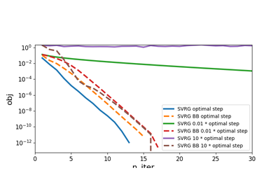
step_type : {‘fixed’, ‘bb’}, default=’fixed’

How step will evoluate over stime

• if 'fixed' step will remain equal to the given step accross all iterations. This is the fastest solution if the optimal step is known.

• if 'bb' step will be chosen given Barzilai Borwein rule. This choice is much more adaptive and should be used if optimal step if difficult to obtain.

print_every : int, default=1

Print history information every time the iteration number is a multiple of print_every. Used only is verbose is True

record_every : int, default=1

Save history information every time the iteration number is a multiple of record_every

Attributes:

model : Model

The model used by the solver, passed with the set_model method

prox : Prox

Proximal operator used by the solver, passed with the set_prox method

solution : numpy.array, shape=(n_coeffs,)

Minimizer found by the solver

history : dict-like

A dict-type of object that contains history of the solver along iterations. It should be accessed using the get_history method

time_start : str

Start date of the call to solve()

time_elapsed : float

Duration of the call to solve(), in seconds

time_end : str

End date of the call to solve()

dtype : {'float64', 'float32'}, default=’float64’

Type of the arrays used. This value is set from model and prox dtypes.

References

• L. Xiao and T. Zhang, A proximal stochastic gradient method with progressive variance reduction, SIAM Journal on Optimization (2014)

• Tan, C., Ma, S., Dai, Y. H., & Qian, Y. Barzilai-Borwein step size for stochastic gradient descent. Advances in Neural Information Processing Systems (2016)

• Mania, H., Pan, X., Papailiopoulos, D., Recht, B., Ramchandran, K. and Jordan, M.I., 2015. Perturbed iterate analysis for asynchronous stochastic optimization.

Examples using tick.solver.SVRG¶