`tick.hawkes`¶

This module proposes a comprehensive set of tools for the inference and the simulation of Hawkes processes, with both parametric and non-parametric estimation techniques and flexible tools for simulation.

Contents

1. Introduction
2. Learners
3. Point process simulation
4. Models for inference

1. Introduction¶

A Hawkes process is a \(D\)-dimensional counting process \(N(t) = (N_1(t) \cdots N_D(t))\), where each coordinate is a counting process \(N_i(t) = \sum_{k \geq 1} \mathbf 1_{t_{i, k} \leq t}\), with \(t_{i, 1}, t_{i, 2}, \ldots\) being the ticks or timestamps observed on component \(i\). The intensity of \(N\) is given by

\[\lambda_i(t) = \mu_i + \sum_{j=1}^D \sum_{k \ : \ t_{j, k} < t} \phi_{ij}(t - t_{j, k})\]

for \(i = 1, \ldots, D\). Such an intensity induces a cluster effect, namely activity one a node \(j\) induces intensity on another node \(i\), with an impact encoded by the kernel function \(\phi_{ij}\). In the the above formula, we have

\(D\) is the number of nodes
\(\mu_i\) are the baseline intensities
\(\phi_{ij}\) are the kernels.

Note that different choices for the shape of the kernels correspond to different models, described below, and two strategies for parametric inference are available, either least-squares estimation or maximum likelihood estimation, both with several choices of penalization.

2. Learners¶

This module proposes learners, that are meant to be very user friendly and are most of the time good enough to infer Hawkes processes based on data, with both parametric and non-parametric approaches.

2.1. Parametric Hawkes learners¶

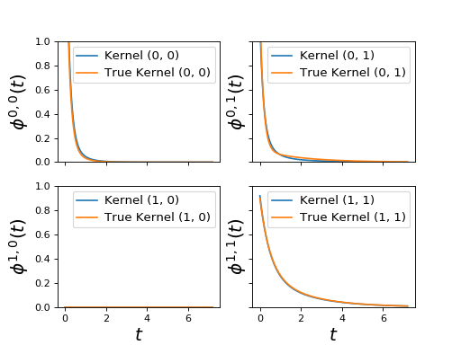
One way to infer Hawkes processes is to suppose that their kernels have a parametric shape. A standard assumption is an exponential parametrization since it allows very fast computations, thanks to tricky recurrence formulas. The following learners propose in their parameters several choices of penalization and solvers.

`HawkesExpKern`(decays[, gofit, penalty, C, …])	Hawkes process learner for exponential kernels with fixed and given decays, with many choices of penalization and solvers.
`HawkesSumExpKern`(decays[, penalty, C, …])	Hawkes process learner for sum-exponential kernels with fixed and given decays, with many choices of penalization and solvers.
`HawkesADM4`(decay[, C, lasso_nuclear_ratio, …])	A class that implements parametric inference for Hawkes processes with an exponential parametrisation of the kernels and a mix of Lasso and nuclear regularization
`HawkesSumGaussians`(max_mean_gaussian[, …])	A class that implements parametric inference for Hawkes processes with parametrisation of the kernels as sum of Gaussian basis functions and a mix of Lasso and group-lasso regularization

Example¶

import matplotlib.pyplot as plt

from tick.plot import plot_hawkes_kernels
from tick.hawkes import SimuHawkesSumExpKernels, SimuHawkesMulti, \
    HawkesSumExpKern

end_time = 1000
n_realizations = 10

decays = [.5, 2., 6.]
baseline = [0.12, 0.07]
adjacency = [[[0, .1, .4], [.2, 0., .2]],
             [[0, 0, 0], [.6, .3, 0]]]

hawkes_exp_kernels = SimuHawkesSumExpKernels(
    adjacency=adjacency, decays=decays, baseline=baseline,
    end_time=end_time, verbose=False, seed=1039)

multi = SimuHawkesMulti(hawkes_exp_kernels, n_simulations=n_realizations)

multi.end_time = [(i + 1) / 10 * end_time for i in range(n_realizations)]
multi.simulate()

learner = HawkesSumExpKern(decays, penalty='elasticnet',
                           elastic_net_ratio=0.8)
learner.fit(multi.timestamps)

fig = plot_hawkes_kernels(learner, hawkes=hawkes_exp_kernels, show=False)

for ax in fig.axes:
    ax.set_ylim([0., 1.])

(Source code, png, hires.png, pdf)

../_images/plot_hawkes_sum_exp_kernels1.png

2.2. Non-parametric Hawkes learners¶

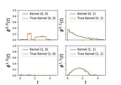
The following Hawkes learners perform non-parametric estimation of the kernels and hence don’t rely on the previous exponential parametrization. However, this methods are less scalable with respect to the number of nodes \(D\). These learners might be used to infer more exotic kernels.

`HawkesEM`([kernel_support, kernel_size, …])	This class is used for performing non parametric estimation of multi-dimensional Hawkes processes based on expectation maximization algorithm.
`HawkesBasisKernels`(kernel_support[, …])	This class is used for performing non parametric estimation of multi-dimensional Hawkes processes based on expectation maximization algorithm and the hypothesis that kernels are linear combinations of some basis kernels.
`HawkesConditionalLaw`([delta_lag, min_lag, …])	This class is used for performing non parametric estimation of multi-dimensional marked Hawkes processes based on conditional laws.
`HawkesCumulantMatching`(integration_support)	This class is used for performing non parametric estimation of multi-dimensional Hawkes processes based cumulant matching.

Example¶

"""
=========================
Fit Hawkes random kernels
=========================

This Hawkes EM (`tick.inference.HawkesEM`) algorithm assume that kernels are
piecewise constant. Hence it can fit basically any kernel form. However it
doesn't scale very well.

It has been originally described in this paper:

Lewis, E., & Mohler, G. (2011).
A nonparametric EM algorithm for multiscale Hawkes processes.
`preprint, 1-16`_.

.. _preprint, 1-16: http://paleo.sscnet.ucla.edu/Lewis-Molher-EM_Preprint.pdf
"""

import numpy as np
import matplotlib.pyplot as plt

from tick.hawkes import (SimuHawkes, HawkesKernelTimeFunc, HawkesKernelExp,
                         HawkesEM)
from tick.base import TimeFunction
from tick.plot import plot_hawkes_kernels

run_time = 30000

t_values1 = np.array([0, 1, 1.5, 2., 3.5], dtype=float)
y_values1 = np.array([0, 0.2, 0, 0.1, 0.], dtype=float)
tf1 = TimeFunction([t_values1, y_values1],
                   inter_mode=TimeFunction.InterConstRight, dt=0.1)
kernel1 = HawkesKernelTimeFunc(tf1)

t_values2 = np.linspace(0, 4, 20)
y_values2 = np.maximum(0., np.sin(t_values2) / 4)
tf2 = TimeFunction([t_values2, y_values2])
kernel2 = HawkesKernelTimeFunc(tf2)

baseline = np.array([0.1, 0.3])

hawkes = SimuHawkes(baseline=baseline, end_time=run_time, verbose=False,
                    seed=2334)

hawkes.set_kernel(0, 0, kernel1)
hawkes.set_kernel(0, 1, HawkesKernelExp(.5, .7))
hawkes.set_kernel(1, 1, kernel2)

hawkes.simulate()

em = HawkesEM(4, kernel_size=16, n_threads=8, verbose=False, tol=1e-3)
em.fit(hawkes.timestamps)

fig = plot_hawkes_kernels(em, hawkes=hawkes, show=False)

for ax in fig.axes:
    ax.set_ylim([0, 1])
plt.show()

(Source code, png, hires.png, pdf)

3. Point process simulation¶

In this section with describe how to simulate point processes and Hawkes processes using tick. First, we need to describe two tools giving flexibility in the simulation of point processes : time functions and kernels for Hawkes process simulation.

3.1. Time function¶

A TimeFunction is a class allowing to define a function on \([0, \infty)\). It uses several types of interpolation to determine its value between two points. It is used for the simulation of an inhomogeneous Poisson process and some Hawkes processes.

base.TimeFunction(values[, border_type, …])

A function depending on time.

Example¶

import matplotlib.pyplot as plt
import numpy as np
from tick.base import TimeFunction
from tick.plot import plot_timefunction

T = np.array([0, 3, 5.9, 8.001], dtype=float)
Y = np.array([2, 4.1, 1, 2], dtype=float)

tf_1 = TimeFunction((T, Y), dt=1.2)
tf_2 = TimeFunction((T, Y), border_type=TimeFunction.BorderContinue,
                    inter_mode=TimeFunction.InterConstRight, dt=0.01)
tf_3 = TimeFunction((T, Y), border_type=TimeFunction.BorderConstant,
                    inter_mode=TimeFunction.InterConstLeft, border_value=3)

time_functions = [tf_1, tf_2, tf_3]

_, ax_list = plt.subplots(1, 3, figsize=(14, 4), sharey=True)

for tf, ax in zip(time_functions, ax_list):
    plot_timefunction(tf_1, ax=ax)
    ax.set_ylim([-0.5, 6.0])
plt.show()

(Source code, png, hires.png, pdf)

3.2. Kernels for Hawkes process simulation¶

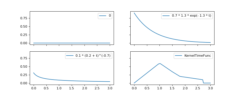
A Hawkes process is defined through its kernels which are functions defined on \([0, \infty)\). The following kernels are available for simulation.

`HawkesKernel0`()	Hawkes zero kernel
`HawkesKernelExp`(intensity, decay)	Hawkes kernel with exponential decay
`HawkesKernelSumExp`(intensities, decays)	Hawkes kernel with sum exponential decays
`HawkesKernelPowerLaw`(multiplier, cutoff, …)	Hawkes kernel for power law
`HawkesKernelTimeFunc`([time_function, …])	Hawkes kernel defined by an arbitrary time function.

Example¶

import numpy as np
import matplotlib.pyplot as plt

from tick.hawkes import HawkesKernel0, HawkesKernelExp, HawkesKernelPowerLaw, \
    HawkesKernelTimeFunc

kernel_0 = HawkesKernel0()
kernel_exp = HawkesKernelExp(.7, 1.3)
kernel_pl = HawkesKernelPowerLaw(.1, .2, 0.7)

t_values = np.array([0, 1, 1.5, 1.8, 2.7])
y_values = np.array([0, .6, .34, .2, .1])
kernel_tf = HawkesKernelTimeFunc(t_values=t_values, y_values=y_values)

kernels = [[kernel_0, kernel_exp], [kernel_pl, kernel_tf]]

fig, ax = plt.subplots(2, 2, sharex=True, sharey=True, figsize=(10, 4))

t_values = np.linspace(0, 3, 100)
for i in range(2):
    for j in range(2):
        ax[i, j].plot(t_values, kernels[i][j].get_values(t_values),
                      label=kernels[i][j])
        ax[i, j].legend()
plt.show()

(Source code, png, hires.png, pdf)

3.3. Poisson processes¶

Both homogeneous and inhomogeneous Poisson process might be simulated with tick thanks to the following classes.

`SimuPoissonProcess`(intensities[, end_time, …])	Homogeneous Poisson process simulation
`SimuInhomogeneousPoisson`(intensities_functions)	Inhomogeneous Poisson process simulation

Examples¶

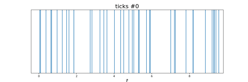
A Poisson process with constant intensity

from tick.hawkes import SimuPoissonProcess
from tick.plot import plot_point_process

run_time = 10
intensity = 5

poi = SimuPoissonProcess(intensity, end_time=run_time, verbose=False)
poi.simulate()
plot_point_process(poi)

(Source code, png, hires.png, pdf)

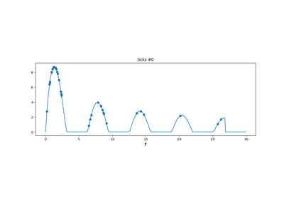
../_images/plot_poisson_constant_intensity1.png

A Poisson process with variable intensity. In this case, the intensity is defined through a tick.base.TimeFunction

"""
========================================
Inhomogeneous Poisson process simulation
========================================

This example show how to simulate any inhomogeneous Poisson process. Its 
intensity is modeled through `tick.base.TimeFunction`
"""

import numpy as np
from tick.base import TimeFunction

from tick.plot import plot_point_process
from tick.hawkes import SimuInhomogeneousPoisson

run_time = 30

T = np.arange((run_time * 0.9) * 5, dtype=float) / 5
Y = np.maximum(
    15 * np.sin(T) * (np.divide(np.ones_like(T),
                                np.sqrt(T + 1) + 0.1 * T)), 0.001)

tf = TimeFunction((T, Y), dt=0.01)

# We define a 1 dimensional inhomogeneous Poisson process with the
# intensity function seen above
in_poi = SimuInhomogeneousPoisson([tf], end_time=run_time, verbose=False)

# We activate intensity tracking and launch simulation
in_poi.track_intensity(0.1)
in_poi.simulate()

# We plot the resulting inhomogeneous Poisson process with its
# intensity and its ticks over time
plot_point_process(in_poi)

(Source code, png, hires.png, pdf)

../_images/plot_poisson_inhomogeneous2.png

3.4. Hawkes processes¶

Simulation of Hawkes processes can be done using the following classes. The main class SimuHawkes might use any type of kernels and will perform simulation. For some specific cases there are some classes dedicated to a type of kernel: exponential or sum of exponential kernels.

`SimuHawkes`([kernels, baseline, n_nodes, …])	Hawkes process simulation
`SimuHawkesExpKernels`(adjacency, decays[, …])	Hawkes process with exponential kernels simulation
`SimuHawkesSumExpKernels`(adjacency, decays[, …])	Hawkes process with sum-exponential kernels simulation

"""
1 dimensional Hawkes process simulation
=======================================
"""

from tick.plot import plot_point_process
from tick.hawkes import SimuHawkes, HawkesKernelSumExp
import matplotlib.pyplot as plt

run_time = 40

hawkes = SimuHawkes(n_nodes=1, end_time=run_time, verbose=False, seed=1398)
kernel = HawkesKernelSumExp([.1, .2, .1], [1., 3., 7.])
hawkes.set_kernel(0, 0, kernel)
hawkes.set_baseline(0, 1.)

dt = 0.01
hawkes.track_intensity(dt)
hawkes.simulate()
timestamps = hawkes.timestamps
intensity = hawkes.tracked_intensity
intensity_times = hawkes.intensity_tracked_times

_, ax = plt.subplots(1, 2, figsize=(16, 4))
plot_point_process(hawkes, n_points=50000, t_min=2, max_jumps=10, ax=ax[0])
plot_point_process(hawkes, n_points=50000, t_min=2, t_max=20, ax=ax[1])

(Source code, png, hires.png, pdf)

"""
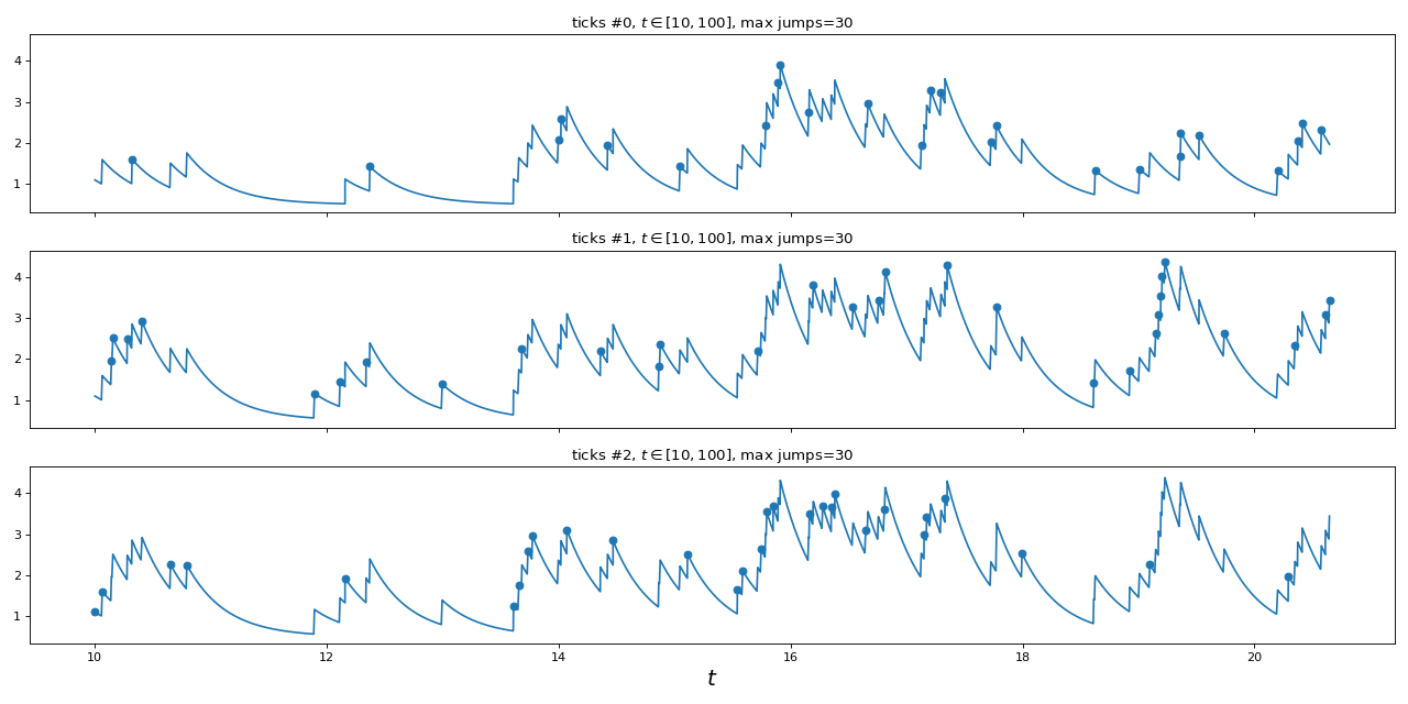
Simulation of 3-dimensional hawkes process
==========================================
"""
import numpy as np
import matplotlib.pyplot as plt

from tick.hawkes import SimuHawkesExpKernels
from tick.plot import plot_point_process

n_nodes = 3  # dimension of the Hawkes process
adjacency = 0.2 * np.ones((n_nodes, n_nodes))
adjacency[0, 1] = 0
decays = 3 * np.ones((n_nodes, n_nodes))
baseline = 0.5 * np.ones(n_nodes)
hawkes = SimuHawkesExpKernels(adjacency=adjacency, decays=decays,
                              baseline=baseline, verbose=False, seed=2398)

run_time = 100
hawkes.end_time = run_time
dt = 0.01
hawkes.track_intensity(dt)
hawkes.simulate()

fig, ax = plt.subplots(n_nodes, 1, figsize=(16, 8), sharex=True, sharey=True)
plot_point_process(hawkes, n_points=50000, t_min=10, max_jumps=30, ax=ax)
fig.tight_layout()

(Source code, png, hires.png, pdf)

../_images/plot_hawkes_multidim_simu1.png

4. Models for inference¶

The following models can be used with a solver to implement cases potentially not covered in 2. Learners. Note that these models are used internally in the learners and feature least-squares and log-likelihood goodness-of-fit for parametric Hawkes models with an exponential kernel or a sum of exponential kernels.

`ModelHawkesExpKernLeastSq`(decays[, approx, …])	Hawkes process model exponential kernels with fixed and given decays.
`ModelHawkesExpKernLogLik`(decay[, n_threads])	Hawkes process model exponential kernels with fixed and given decay.
`ModelHawkesSumExpKernLeastSq`(decays[, …])	Hawkes process model for sum-exponential kernels with fixed and given decays.
`ModelHawkesSumExpKernLogLik`(decays[, n_threads])	Hawkes process model for sum of exponential kernels with fixed and given decays.

tick.hawkes¶

1. Introduction¶

2. Learners¶

2.1. Parametric Hawkes learners¶

Example¶

2.2. Non-parametric Hawkes learners¶

Example¶

3. Point process simulation¶

3.1. Time function¶

Example¶

3.2. Kernels for Hawkes process simulation¶

Example¶

3.3. Poisson processes¶

Examples¶

3.4. Hawkes processes¶

4. Models for inference¶

`tick.hawkes`¶