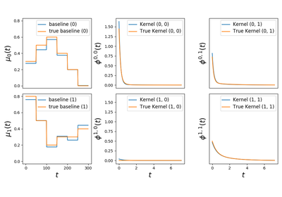
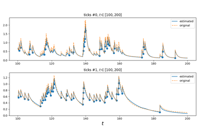
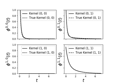
tick.hawkes.HawkesSumExpKern¶

class tick.hawkes.HawkesSumExpKern(decays, penalty='l2', C=1000.0, n_baselines=1, period_length=None, solver='agd', step=None, tol=1e-05, max_iter=100, verbose=False, print_every=10, record_every=10, elastic_net_ratio=0.95, random_state=None)[source]¶

Hawkes process learner for sum-exponential kernels with fixed and given decays, with many choices of penalization and solvers.

Hawkes processes are point processes defined by the intensity:

\[\forall i \in [1 \dots D], \quad \lambda_i(t) = \mu_i(t) + \sum_{j=1}^D \sum_{t_k^j < t} \phi_{ij}(t - t_k^j)\]

where

\(D\) is the number of nodes
\(\mu_i(t)\) are the baseline intensities
\(\phi_{ij}\) are the kernels
\(t_k^j\) are the timestamps of all events of node \(j\)

and with an sum-exponential parametrisation of the kernels

\[\phi_{ij}(t) = \sum_{u=1}^{U} \alpha^u_{ij} \beta^u \exp (- \beta^u t) 1_{t > 0}\]

In our implementation we denote:

Integer \(D\) by the attribute n_nodes
Integer \(U\) by the attribute n_decays
Vector \(\mu \in \mathbb{R}^{D}\) by the attribute baseline
Matrix \(A = (\alpha^u_{ij})_{ij} \in \mathbb{R}^{D \times D \times U}\) by the attribute adjacency
Vector \(\beta \in \mathbb{R}^{U}\) by the parameter decays. This parameter is given to the model

Parameters

decays : np.ndarray, shape=(n_decays, )

The decays used in the exponential kernels.

n_baselines : int, default=1

In this hawkes learner baseline is supposed to be either constant or piecewise constant. If n_baseline > 1 then piecewise constant setting is enabled. In this case \(\mu_i(t)\) is piecewise constant on intervals of size period_length / n_baselines and periodic.

period_length : float, default=None

In piecewise constant setting this denotes the period of the piecewise constant baseline function.

C : float, default=1e3

Level of penalization

penalty : {‘l1’, ‘l2’, ‘elasticnet’, ‘none’} default=’l2’

The penalization to use. Default is ridge penalization.

solver : {‘gd’, ‘agd’, ‘bfgs’, ‘svrg’}, default=’agd’

The name of the solver to use

step : float, default=None

Initial step size used for learning. Used in ‘gd’, ‘agd’, ‘sgd’ and ‘svrg’ solvers

tol : float, default=1e-5

The tolerance of the solver (iterations stop when the stopping criterion is below it). If not reached the solver does max_iter iterations

max_iter : int, default=100

Maximum number of iterations of the solver

verbose : bool, default=False

If True, we verbose things, otherwise the solver does not print anything (but records information in history anyway)

print_every : int, default=10

Print history information when n_iter (iteration number) is a multiple of print_every

record_every : int, default=10

Record history information when n_iter (iteration number) is a multiple of record_every

elastic_net_ratio : float, default=0.95

Ratio of elastic net mixing parameter with 0 <= ratio <= 1.

For ratio = 0 this is ridge (L2 squared) regularization.

For ratio = 1 this is lasso (L1) regularization.

For 0 < ratio < 1, the regularization is a linear combination of L1 and L2.

Used in ‘elasticnet’ penalty

random_state : int seed, or None (default)

The seed that will be used by stochastic solvers. If None, a random seed will be used (based on timestamp and other physical metrics). Used in ‘sgd’, and ‘svrg’ solvers

Attributes

n_nodes : int

Number of nodes / components in the Hawkes model

baseline : np.array, shape=(n_nodes,)

Inferred baseline of each component’s intensity

adjacency : np.ndarray, shape=(n_nodes, n_nodes, n_decays)

Inferred adjacency matrix

coeffs : np.array, shape=(n_nodes + n_nodes * n_nodes * n_decays, )

Raw coefficients of the model. Row stack of self.baseline and self.adjacency

__init__(decays, penalty='l2', C=1000.0, n_baselines=1, period_length=None, solver='agd', step=None, tol=1e-05, max_iter=100, verbose=False, print_every=10, record_every=10, elastic_net_ratio=0.95, random_state=None)¶

estimated_intensity(events, intensity_track_step, end_time=None)¶

Value of intensity for a given realization with the fitted parameters

Parameters

events : list of np.ndarray, default = None

One Hawkes processes realization, a list of n_node for each component of the Hawkes. Namely events[i] contains a one-dimensional numpy.array of the events’ timestamps of component i.

intensity_track_step : float, default = None

How often the intensity should be computed

end_time : float, default = None

End time of hawkes process. If None, it will be set to realization’s latest time.

Returns

tracked_intensity : list of np.array

intensity values for all components

intensity_tracked_times : np.array

Times at wich intensity has been recorded

fit(events: list, start=None)¶

Fit the model according to the given training data.

Parameters

events : list of np.array

The events of each component of the Hawkes. Namely events[j] contains a one-dimensional numpy.array of the events’ timestamps of component j

start : np.array or float, default=None

If np.array, the initial coeffs coefficients passed to the solver, ie. the optimization algorithm. If a float is given, the initial point will be the vector filled with this float. If None it will be automatically chosen.

Returns

output : LearnerHawkesParametric

The current instance of the Learner

get_kernel_norms()¶

Computes kernel norms. This makes our learner compliant with tick.plot.plot_hawkes_kernel_norms API

Returns: norms : np.ndarray, shape=(n_nodes, n_nodes)

2d array in which each entry i, j corresponds to the norm of kernel i, j

get_kernel_supports()¶

Computes kernel support. This makes our learner compliant with tick.plot.plot_hawkes_kernels API

Returns: output : np.ndarray, shape=(n_nodes, n_nodes)

2d array in which each entry i, j corresponds to the support of kernel i, j

get_kernel_values(i, j, abscissa_array)¶

Computes value of the specified kernel on given time values. This makes our learner compliant with tick.plot.plot_hawkes_kernels API

Parameters

i : int

First index of the kernel

j : int

Second index of the kernel

abscissa_array : np.ndarray, shape=(n_points, )

1d array containing all the times at which this kernel will computes it value

Returns

output : np.ndarray, shape=(n_points, )

1d array containing the values of the specified kernels at the given times.

plot_estimated_intensity(events, n_points=10000, plot_nodes=None, t_min=None, t_max=None, intensity_track_step=None, max_jumps=None, show=True, ax=None)¶

Plot value of intensity for a given realization with the fitted parameters

eventslist of np.ndarray, default = None: One Hawkes processes realization, a list of n_node for each component of the Hawkes. Namely events[i] contains a one-dimensional numpy.array of the events’ timestamps of component i.
n_pointsint, default=10000: Number of points used for intensity plot.
plot_nodeslist of int, default=`None`: List of nodes that will be plotted. If None, all nodes are considered
t_minfloat, default=`None`: If not None, time at which plot will start
t_maxfloat, default=`None`: If not None, time at which plot will stop
intensity_track_stepfloat, default=`None`: Defines how often intensity will be computed. If this is too low, computations might be long. By default, a value will be extrapolated from (t_max - t_min) / n_points.
max_jumpsint, default=`None`: If not None, maximum of jumps per coordinate that will be plotted. This is useful when plotting big point processes to ensure a only readable part of them will be plotted
showbool, default=`True`: if True, show the plot. Otherwise an explicit call to the show function is necessary. Useful when superposing several plots.
axlist of matplotlib.axes, default=None: If not None, the figure will be plot on this axis and show will be set to False.

score(events=None, end_times=None, baseline=None, adjacency=None)[source]¶

Compute score metric Score metric is log likelihood (the higher the better)

Parameters

events : list of list of np.ndarray, default = None

List of Hawkes processes realizations used to measure score. Each realization of the Hawkes process is a list of n_node for each component of the Hawkes. Namely events[i][j] contains a one-dimensional numpy.array of the events’ timestamps of component j of realization i. If only one realization is given, it will be wrapped into a list If None, events given while fitting model will be used

end_times : np.ndarray or float, default = None

List of end time of all hawkes processes used to measure score. If None, it will be set to each realization’s latest time. If only one realization is provided, then a float can be given.

baseline : np.ndarray, shape=(n_nodes, ), default = None