tick.survival
This module provides some tools for survival analysis. It provides a learner for Cox regression and a model for Self Control Case Series (SCCS).
1. Learners
For now, this module provides only a learner for Cox regression for proportional hazards, using the partial likelihood. It also provides Nelson-Aalen and Kaplan-Meier estimators.
|
Cox regression learner, using the partial Cox likelihood for proportional risks, with many choices of penalization. |
|
Computes the Nelson-Aalen cumulative hazard rate estimation given by: |
|
Computes the Kaplan-Meier survival function estimation given by: |
|
ConvSCCS learner, estimates lagged features effect using TV and Group L1 penalties. |
|
BatchConvSCCS provides parallel batch solving for ConvSCCS k_fold |
|
StreamConvSCCS provides parallel solving for k_fold and bootstrap ConvSCCS |
2. Models
The following models can be used with solvers for inference. Note that
ModelCoxRegPartialLik cannot
be used for now with a stochastic solver, while we can with ModelSCCS.
Partial likelihood of the Cox regression model (proportional hazards). |
|
|
Discrete-time Self Control Case Series (SCCS) likelihood. |
3. Simulation
We provide tools for the simulation of datasets, for both right-censored
durations following a proportional risks model, and a SCCS model.
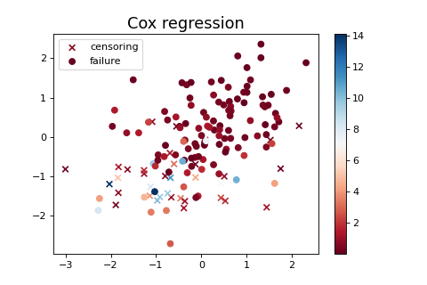
SimuCoxReg generates data in the form of i.i.d triplets \((x_i, t_i, c_i)\)
for \(i=1, \ldots, n\), where \(x_i \in \mathbb R^d\) is a features vector,
\(t_i \in \mathbb R_+\) is the survival time and \(c_i \in \{ 0, 1 \}\) is the
indicator of right censoring.
Note that \(c_i = 1\) means that \(t_i\) is a failure time
while \(c_i = 0\) means that \(t_i\) is a censoring time.
|
Simulation of a Cox regression for proportional hazards |
|
Simulation of a Self Control Case Series (SCCS) model. |
Example
"""
==============================
Cox regression data simulation
==============================
Generates Cox Regression realization given a weight vector
"""
import matplotlib.pyplot as plt
import numpy as np
from tick.survival import SimuCoxReg
n_samples = 150
weights = np.array([0.3, 1.2])
seed = 123
simu_coxreg = SimuCoxReg(weights, n_samples=n_samples, seed=123, verbose=False)
X, T, C = simu_coxreg.simulate()
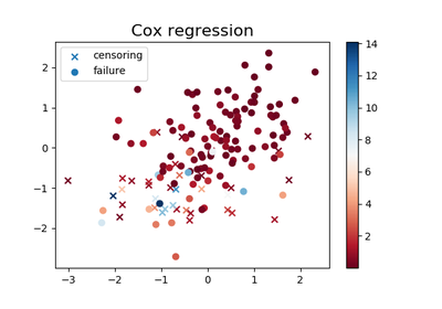
plt.figure(figsize=(6, 4))
plt.scatter(*X[C == 0].T, c=T[C == 0], cmap='RdBu', marker="x",
label="censoring")
plt.scatter(*X[C == 1].T, c=T[C == 1], cmap='RdBu', marker="o",
label="failure")
plt.colorbar()
plt.legend(loc='upper left')
plt.title('Cox regression', fontsize=16)
(Source code, png, hires.png, pdf)
"""
====================================================================
ConvSCCS cross validation on simulated longitudinal features example
====================================================================
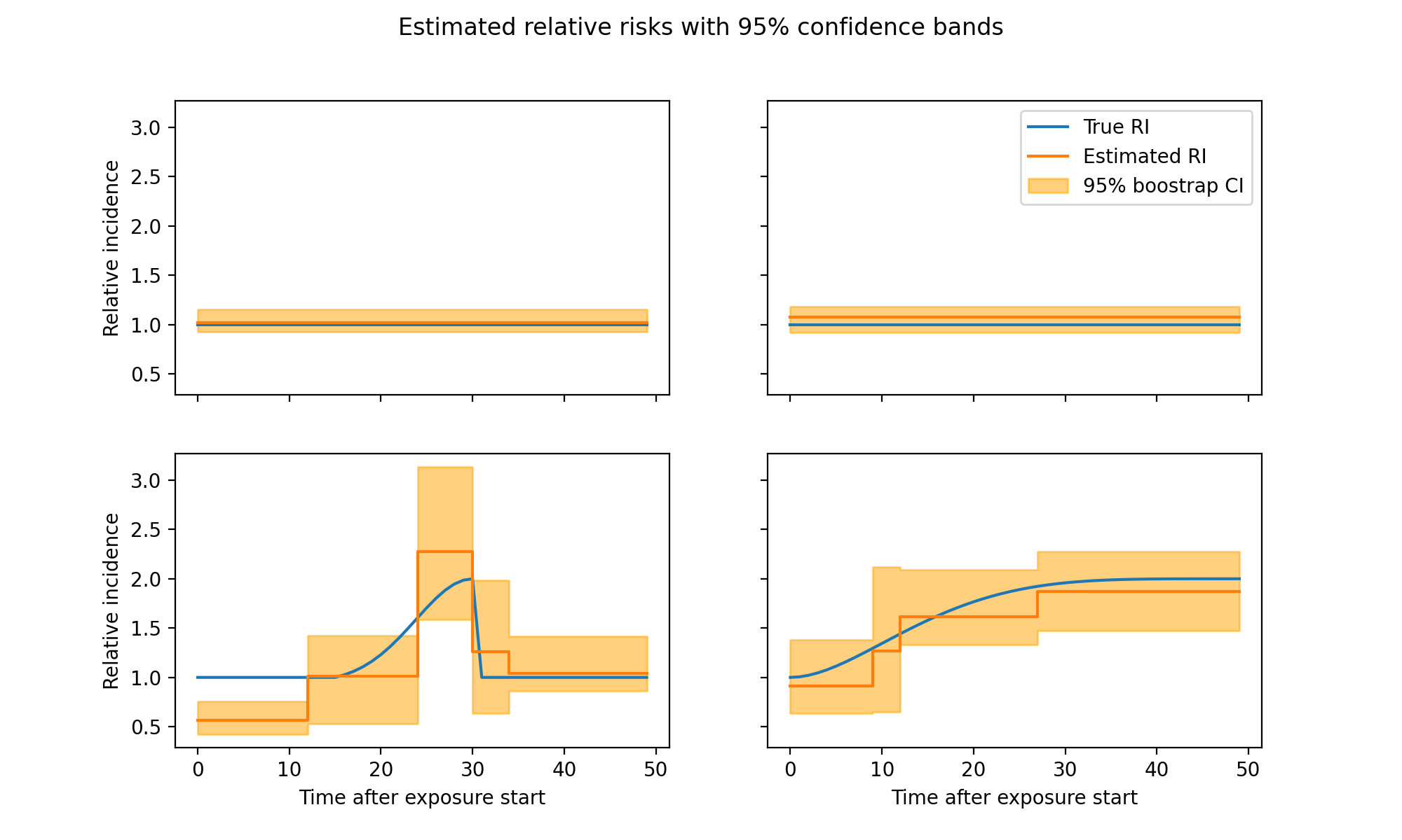
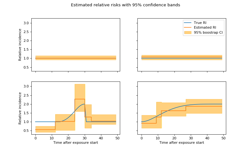
In this example we simulate longitudinal data with preset relative incidence
for each feature. We then perform a cross validation of the ConvSCCS model
and compare the estimated coefficients to the relative incidences used for
the simulation.
"""
import numpy as np
from scipy.sparse import csr_matrix, hstack
from matplotlib import cm
import matplotlib.pylab as plt
from tick.survival.simu_sccs import CustomEffects
from tick.survival import SimuSCCS, ConvSCCS
from mpl_toolkits.axes_grid1 import make_axes_locatable
# Simulation parameters
seed = 0
lags = 49
n_samples = 2000
n_intervals = 750
n_corr = 3
# Relative incidence functions used for the simulation
ce = CustomEffects(lags + 1)
null_effect = [ce.constant_effect(1)] * 2
intermediate_effect = ce.bell_shaped_effect(2, 30, 15, 15)
late_effects = ce.increasing_effect(2, curvature_type=4)
sim_effects = [*null_effect, intermediate_effect, late_effects]
n_features = len(sim_effects)
n_lags = np.repeat(lags, n_features).astype('uint64')
coeffs = [np.log(c) for c in sim_effects]
# Time drift (age effect) used for the simulations.
time_drift = lambda t: np.log(8 * np.sin(.01 * t) + 9)
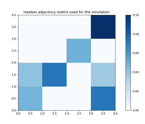
# Simaltion of the features.
sim = SimuSCCS(n_samples, n_intervals, n_features, n_lags,
time_drift=time_drift, coeffs=coeffs, seed=seed,
n_correlations=n_corr, verbose=False)
features, censored_features, labels, censoring, coeffs = sim.simulate()
# Plot the Hawkes kernel matrix used to generate the features.
fig, ax = plt.subplots(figsize=(7, 6))
heatmap = ax.pcolor(sim.hawkes_exp_kernels.adjacency, cmap=cm.Blues)
divider = make_axes_locatable(ax)
cax = divider.append_axes("right", size="5%", pad=0.5)
fig.colorbar(heatmap, cax=cax)
ax.set_title('Hawkes adjacency matrix used for the simulation')
plt.show()
(Source code, png, hires.png, pdf)

## Add age_groups features to feature matrices.
agegrps = [0, 125, 250, 375, 500, 625, 750]
n_agegrps = len(agegrps) - 1

feat_agegrp = np.zeros((n_intervals, n_agegrps))
for i in range(n_agegrps):
    feat_agegrp[agegrps[i]:agegrps[i + 1], i] = 1

feat_agegrp = csr_matrix(feat_agegrp)
features = [hstack([f, feat_agegrp]).tocsr() for f in features]
censored_features = [
    hstack([f, feat_agegrp]).tocsr() for f in censored_features
]
n_lags = np.hstack([n_lags, np.zeros(n_agegrps)])

# Learning
# Example code for cross validation
# start = time()
# learner = ConvSCCS(n_lags=n_lags.astype('uint64'),
#                    penalized_features=np.arange(n_features),
#                    random_state=42)
# C_TV_range = (1, 4)
# C_L1_range = (2, 5)
# _, cv_track = learner.fit_kfold_cv(features, labels, censoring,
#                                    C_TV_range, C_L1_range,
#                                    confidence_intervals=True,
#                                    n_samples_bootstrap=20, n_cv_iter=50)
# elapsed_time = time() - start
# print("Elapsed time (model training): %.2f seconds \n" % elapsed_time)
# print("Best model hyper parameters: \n")
# print("C_tv : %f \n" % cv_track.best_model['C_tv'])
# print("C_group_l1 : %f \n" % cv_track.best_model['C_group_l1'])
# cv_track.plot_cv_report(35, 45)
# plt.show()
# confidence_intervals = cv_track.best_model['confidence_intervals']

# using the parameters resulting from cross-validation
learner = ConvSCCS(
    n_lags=n_lags.astype('uint64'), penalized_features=np.arange(n_features),
    random_state=42, C_tv=270.2722840570933, C_group_l1=5216.472772625124)

_, confidence_intervals = learner.fit(features, labels, censoring,
                                      confidence_intervals=True,
                                      n_samples_bootstrap=20)

# Plot estimated parameters
# get bootstrap confidence intervals
refitted_coeffs = confidence_intervals['refit_coeffs']
lower_bound = confidence_intervals['lower_bound']
upper_bound = confidence_intervals['upper_bound']

n_rows = int(np.ceil(n_features / 2))
remove_last_plot = (n_features % 2 != 0)

fig, axarr = plt.subplots(n_rows, 2, sharex=True, sharey=True, figsize=(10, 6))
y = confidence_intervals['refit_coeffs']
lb = confidence_intervals['lower_bound']
ub = confidence_intervals['upper_bound']
for i, c in enumerate(y[:-6]):
    ax = axarr[i // 2][i % 2]
    l = n_lags[i]
    ax.plot(np.exp(coeffs[i]), label="True RI")
    ax.step(np.arange(l + 1), np.exp(c), label="Estimated RI")
    ax.fill_between(
        np.arange(l + 1), np.exp(lb[i]), np.exp(ub[i]), alpha=.5,
        color='orange', step='pre', label="95% boostrap CI")
plt.suptitle('Estimated relative risks with 95% confidence bands')
axarr[0][1].legend(loc='best')
[ax[0].set_ylabel('Relative incidence') for ax in axarr]
[ax.set_xlabel('Time after exposure start') for ax in axarr[-1]]
if remove_last_plot:
    fig.delaxes(axarr[-1][-1])
plt.show()
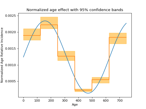
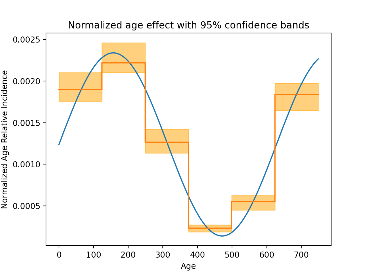
normalize = lambda x: x / np.sum(x)
m = np.repeat(np.hstack(refitted_coeffs[-6:]), 125)
lb = np.repeat(np.hstack(lower_bound[-6:]), 125)
ub = np.repeat(np.hstack(upper_bound[-6:]), 125)
plt.figure()
plt.plot(
    np.arange(n_intervals),
    normalize(np.exp(time_drift(np.arange(n_intervals)))))
plt.step(np.arange(n_intervals), normalize(np.exp(m)))
plt.fill_between(
    np.arange(n_intervals),
    np.exp(lb) / np.exp(m).sum(),
    np.exp(ub) / np.exp(m).sum(), alpha=.5, color='orange', step='pre')
plt.xlabel('Age')
plt.ylabel('Normalized Age Relative Incidence')
plt.title("Normalized age effect with 95% confidence bands")
plt.show()