tick.solver
This is a solver toolbox, which is used to train almost all models in tick.
It features two types of solvers: deterministic and stochastic.
Deterministic solvers use a full pass over data at each iteration, while
stochastic solvers make epoch_size iterations within each iteration.
Most of the optimization problems considered here can be written as
where \(f\) is a goodness-of-fit term, which depends on the model considered, and \(g\) is a function penalizing \(w\) (see the tick.prox module).
1. The solver class API
All the solvers have a set_model method, which corresponds to the function
\(f\) to pass the model to be trained, and a set_prox method to pass
the penalization, which corresponds to the \(g\).
The solver is launched using the solve method to which a starting point and
eventually a step-size can be given. Here is an example, another example is
also given below.
import numpy as np
from tick.linear_model import SimuLogReg, ModelLogReg
from tick.simulation import weights_sparse_gauss
from tick.solver import SVRG
from tick.prox import ProxElasticNet

n_samples, n_features = 5000, 10
weights0 = weights_sparse_gauss(n_weights=n_features, nnz=3)
intercept0 = 1.
X, y = SimuLogReg(weights0, intercept=intercept0, seed=123,
                  n_samples=n_samples, verbose=False).simulate()

model = ModelLogReg(fit_intercept=True).fit(X, y)
prox = ProxElasticNet(strength=1e-3, ratio=0.5, range=(0, n_features))

svrg = SVRG(tol=0., max_iter=5, print_every=1).set_model(model).set_prox(prox)
x0 = np.zeros(model.n_coeffs)
minimizer = svrg.solve(x0, step=1 / model.get_lip_max())
print("\nfound minimizer\n", minimizer)
which outputs
Launching the solver SVRG...
  n_iter  |    obj    |  rel_obj
        1 |  5.01e-01 |  5.15e-02
        2 |  4.97e-01 |  8.44e-03
        3 |  4.97e-01 |  5.00e-04
        4 |  4.97e-01 |  2.82e-05
        5 |  4.97e-01 |  7.28e-07

Done solving using SVRG in 0.03281998634338379 seconds

found minimizer
 [ 0.01992683  0.00456966 -0.16595686 -0.08619878  0.01059461  0.6144692
  0.0049031  -0.07767023  0.07550217  1.18493663  0.9424508 ]
Note the argument step=1 / model.get_lip_max()) passed to the solve method that gives
an automatic tuning of the step size.
2. Available solvers
Here is the list of the solvers available in tick. Note that a lot of
details about each solver is available in the classes documentations, linked
below.
Solver |
Class |
|---|---|
Proximal gradient descent |
|
Accelerated proximal gradient descent |
|
Broyden, Fletcher, Goldfarb, and Shannon (quasi-newton) |
|
Self-Concordant Proximal Gradient Descent |
|
Generalized Forward-Backward |
|
Stochastic Gradient Descent |
|
Adaptive Gradient Descent solver |
|
Stochastic Variance Reduced Descent |
|
Stochastic Averaged Gradient Descent |
|
Stochastic Dual Coordinate Ascent |
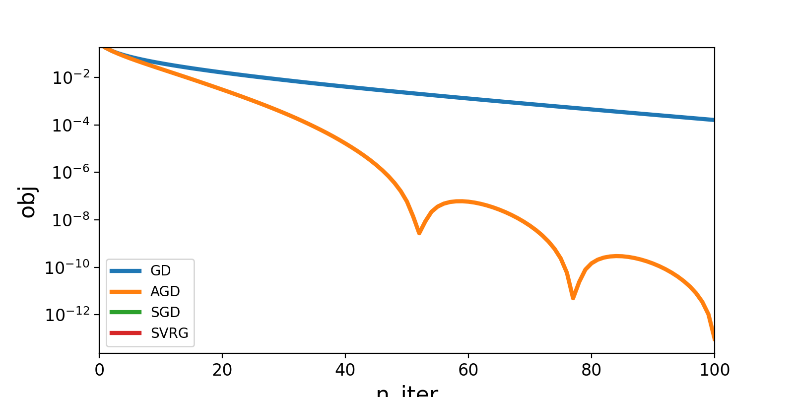
3. Example
Here is an example of combination of a model a prox and a solver to
compare the training time of several solvers for logistic regression with the
elastic-net penalization.
Note that, we specify a range=(0, n_features) so that the intercept is not penalized
(see tick.prox for more details).
import numpy as np
from tick.linear_model import ModelLogReg ,SimuLogReg
from tick.simulation import weights_sparse_gauss
from tick.solver import GD, AGD, SGD, SVRG, SDCA
from tick.prox import ProxElasticNet, ProxL1
from tick.plot import plot_history

n_samples, n_features, = 5000, 50
weights0 = weights_sparse_gauss(n_features, nnz=10)
intercept0 = 0.2
X, y = SimuLogReg(weights=weights0, intercept=intercept0,
                  n_samples=n_samples, seed=123, verbose=False).simulate()

model = ModelLogReg(fit_intercept=True).fit(X, y)
prox = ProxElasticNet(strength=1e-3, ratio=0.5, range=(0, n_features))

solver_params = {'max_iter': 100, 'tol': 0., 'verbose': False}
x0 = np.zeros(model.n_coeffs)

gd = GD(linesearch=False, **solver_params).set_model(model).set_prox(prox)
gd.solve(x0, step=1 / model.get_lip_best())

agd = AGD(linesearch=False, **solver_params).set_model(model).set_prox(prox)
agd.solve(x0, step=1 / model.get_lip_best())

sgd = SGD(**solver_params).set_model(model).set_prox(prox)
sgd.solve(x0, step=500.)

svrg = SVRG(**solver_params).set_model(model).set_prox(prox)
svrg.solve(x0, step=1 / model.get_lip_max())

plot_history([gd, agd, sgd, svrg], log_scale=True, dist_min=True)
(Source code, png, hires.png, pdf)
