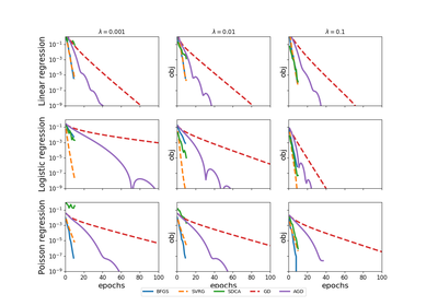
tick.solver.SDCA¶

class tick.solver.SDCA(l_l2sq: float, epoch_size: int = None, rand_type: str = 'unif', tol: float = 1e-10, max_iter: int = 10, verbose: bool = True, print_every: int = 1, record_every: int = 1, seed: int = -1)[source]¶

Stochastic Dual Coordinate Ascent

For the minimization of objectives of the form

\[\frac 1n \sum_{i=1}^n f_i(w^\top x_i) + g(w),\]

where the functions \(f_i\) have smooth gradients and \(g\) is prox-capable. This solver actually requires more than that, since it is working in a Fenchel dual formulation of the primal problem given above. First, it requires that some ridge penalization is used, hence the mandatory parameter l_l2sq below: SDCA will actually minimize the objective

\[\frac 1n \sum_{i=1}^n f_i(x_i^\top w) + g(w) + \frac{\lambda}{2} \| w \|_2^2,\]

where \(\lambda\) is tuned with the l_l2sq (see below). Now, putting \(h(w) = g(w) + \lambda \|w\|_2^2 / 2\), SDCA maximize the Fenchel dual problem

\[D(\alpha) = \frac 1n \sum_{i=1}^n \Bigg[ - f_i^*(-\alpha_i) - \lambda h^*\Big( \frac{1}{\lambda n} \sum_{i=1}^n \alpha_i x_i) \Big) \Bigg],\]

where \(f_i^*\) and \(h^*\) and the Fenchel duals of \(f_i\) and \(h\) respectively. Function \(f = \frac 1n \sum_{i=1}^n f_i\) corresponds to the model.loss method of the model (passed with set_model to the solver) and \(g\) corresponds to the prox.value method of the prox (passed with the set_prox method). One iteration of SDCA corresponds to the following iteration applied epoch_size times:

\[\begin{split}\begin{align*} \delta_i &\gets \arg\min_{\delta} \Big[ \; f_i^*(-\alpha_i - \delta) + w^\top x_i \delta + \frac{1}{2 \lambda n} \| x_i\|_2^2 \delta^2 \Big] \\ \alpha_i &\gets \alpha_i + \delta_i \\ v &\gets v + \frac{1}{\lambda n} \delta_i x_i \\ w &\gets \nabla g^*(v) \end{align*}\end{split}\]

where \(i\) is sampled at random (strategy depends on rand_type) at each iteration. The ridge regularization \(\lambda\) can be tuned with l_l2sq, the seed of the random number generator for generation of samples \(i\) can be seeded with seed. The iterations stop whenever tolerance tol is achieved, or after max_iter epochs (namely max_iter \(\times\) epoch_size iterates). The obtained solution \(w\) is returned by the solve method, and is also stored in the solution attribute of the solver. The dual solution \(\alpha\) is stored in the dual_solution attribute.

Internally, SDCA has dedicated code when the model is a generalized linear model with sparse features, and a separable proximal operator: in this case, each iteration works only in the set of non-zero features, leading to much faster iterates.

Parameters:

l_l2sq : float

Level of L2 penalization. L2 penalization is mandatory for SDCA. Convergence properties of this solver are deeply connected to this parameter, which should be understood as the “step” used by the algorithm.

tol : float, default=1e-10

The tolerance of the solver (iterations stop when the stopping criterion is below it)

max_iter : int, default=10

Maximum number of iterations of the solver, namely maximum number of epochs (by default full pass over the data, unless epoch_size has been modified from default)

verbose : bool, default=True

If True, solver verboses history, otherwise nothing is displayed, but history is recorded anyway

seed : int, default=-1

The seed of the random sampling. If it is negative then a random seed (different at each run) will be chosen.

epoch_size : int, default given by model

Epoch size, namely how many iterations are made before updating the variance reducing term. By default, this is automatically tuned using information from the model object passed through set_model.

rand_type : {‘unif’, ‘perm’}, default=’unif’

How samples are randomly selected from the data

• if 'unif' samples are uniformly drawn among all possibilities

• if 'perm' a random permutation of all possibilities is generated and samples are sequentially taken from it. Once all of them have been taken, a new random permutation is generated

print_every : int, default=1

Print history information every time the iteration number is a multiple of print_every. Used only is verbose is True

record_every : int, default=1

Save history information every time the iteration number is a multiple of record_every

Attributes:

model : Model

The model used by the solver, passed with the set_model method

prox : Prox

Proximal operator used by the solver, passed with the set_prox method

solution : numpy.array, shape=(n_coeffs,)

Minimizer found by the solver

dual_solution : numpy.array

Dual vector corresponding to the primal solution obtained by the solver

history : dict-like

A dict-type of object that contains history of the solver along iterations. It should be accessed using the get_history method

time_start : str

Start date of the call to solve()

time_elapsed : float

Duration of the call to solve(), in seconds

time_end : str

End date of the call to solve()

dtype : {'float64', 'float32'}, default=’float64’

Type of the arrays used. This value is set from model and prox dtypes.

References

• S. Shalev-Shwartz and T. Zhang, Accelerated proximal stochastic dual coordinate ascent for regularized loss minimization, ICML 2014

Examples using tick.solver.SDCA¶