tick.hawkes.HawkesConditionalLaw
- class tick.hawkes.HawkesConditionalLaw(delta_lag=0.1, min_lag=0.0001, max_lag=40, n_quad=50, max_support=40, min_support=0.0001, quad_method='gauss', marked_components=None, delayed_component=None, delay=1e-05, model=None, n_threads=1, claw_method='lin')[source]
This class is used for performing non parametric estimation of multi-dimensional marked Hawkes processes based on conditional laws.
Marked Hawkes processes are point processes defined by the intensity:
\[\forall i \in [1 \dots D], \quad \lambda_i = \mu_i + \sum_{j=1}^D \int \phi_{ij} * f_{ij}(v_j) dN_j\]where
\(D\) is the number of nodes
\(\mu_i\) are the baseline intensities
\(\phi_{ij}\) are the kernels
\(v_j\) are the marks (considered iid) of the process \(N_j\)
\(f_{ij}\) the mark functions supposed to be piece-wise constant on intervals \(I^j(l)\)
The estimation is made from empirical computations of
\[\lim_{\epsilon \rightarrow 0} E [ (N_i[t + lag + \delta + \epsilon] - \Lambda[t + lag + \epsilon]) | N_j[t]=1 \quad \& \quad v_j(t) \in I^j(l) ]\]For all the possible values of \(i\), \(i\) and \(l\). The \(lag\) is sampled on a uniform grid defined by \(\delta\): \(lag = n * \delta\).
Estimation can be performed using several realizations.
- Parameters:
claw_method : {‘lin’, ‘log’}, default=’lin’
Specifies the way the conditional laws are sampled. It can be either:
‘lin’ : sampling is linear on [0, max_lag] using sampling period delta_lag
‘log’ : sampling is semi-log. It uses linear sampling on [0, min_lag] with sampling period delta_lag and log sampling on [min_lag, max_lag] using \(\exp(\delta)\) sampling period.
delta_lag :
float, default=0.1See claw_methods
min_lag :
float, default=1e-4See claw_methods
max_lag :
float, default=40See claw_methods
quad_method : {‘gauss’, ‘lin’, ‘log’}, default=gauss
Sampling used for quadrature
‘gauss’ for gaussian quadrature
‘lin’ for linear quadrature
‘log’ for log quadrature
min_support :
float, default=1e-4Start value of kernel estimation. It is used for ‘log’ quadrature method only, otherwise it is set to 0.
max_support :
float, default=40End value of kernel estimation
n_quad :
intThe number of quadrature points between [min_support, max_support] used for solving the system. Be aware that the complexity increase as this number squared.
n_threads :
int, default=1Number of threads used for parallel computation.
if
int <= 0: the number of physical cores available on the CPUotherwise the desired number of threads
- Attributes:
n_nodes :
intNumber of nodes of the estimated Hawkes process
n_realizations :
intNumber of given realizations
baseline : np.ndarray, shape=(n_nodes,)
Estimation of the baseline
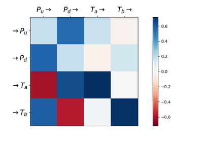
kernels_norms : np.ndarray, shape=(n_nodes, n_nodes)
L1 norm matrix of the kernel norms
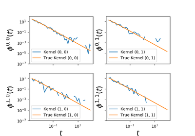
kernels : list of list
Kernel’s estimation on the quadrature points
mean_intensity : list of
floatThe estimated mean intensity
symmetries1d : list of 2-tuple
List of component index pairs for imposing symmetries on the mean intensity (e.g,
[(0,1),(2,3)]means that the mean intensity of the components 0 and 1 must be the same and the mean intensity of the components 2 and 3 also Can be set using can be set using theset_modelmethod.symmetries2d : list of 2-tuple of 2-tuple
List of kernel coordinates pairs to impose symmetries on the kernel matrix (e.g.,
[[(0,0),(1,1)],[(1,0),(0,1)]]for a bidiagonal kernel in dimension 2) Can be set using can be set using theset_modelmethod.mark_functions : list of 2-tuple
The mark functions as a list (lexical order on i,j and l, see below)
References
Bacry, E., & Muzy, J. F. (2014). Second order statistics characterization of Hawkes processes and non-parametric estimation. arXiv preprint arXiv:1401.0903.