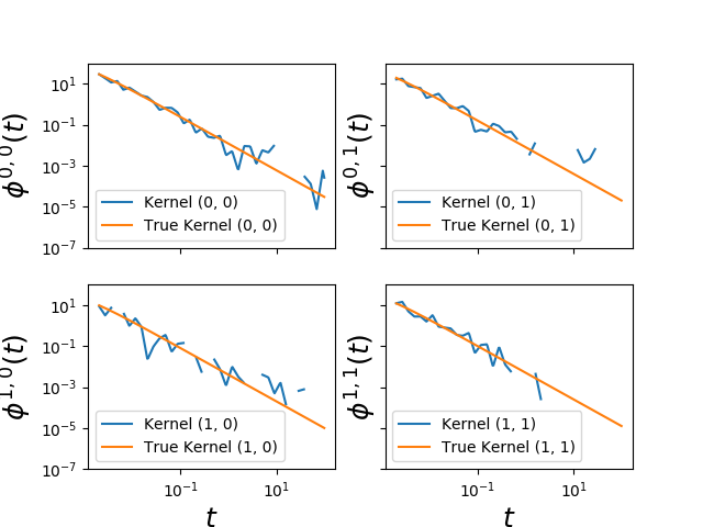
Fit Hawkes power law kernels
This Hawkes learner based on conditional laws
(tick.inference.HawkesConditionalLaw) is able to fit Hawkes power law
kernels commonly found in finance applications.
It has been introduced in the following paper:
Bacry, E., & Muzy, J. F. (2014). Second order statistics characterization of Hawkes processes and non-parametric estimation. arXiv preprint arXiv:1401.0903.
Python source code: plot_hawkes_conditional_law.py
import numpy as np
import matplotlib.pyplot as plt

from tick.hawkes import SimuHawkes, HawkesKernelPowerLaw, HawkesConditionalLaw
from tick.plot import plot_hawkes_kernels

multiplier = np.array([0.012, 0.008, 0.004, 0.005])
cutoff = 0.0005
exponent = 1.3

support = 2000

hawkes = SimuHawkes(
    kernels=[[
        HawkesKernelPowerLaw(multiplier[0], cutoff, exponent, support),
        HawkesKernelPowerLaw(multiplier[1], cutoff, exponent, support)
    ], [
        HawkesKernelPowerLaw(multiplier[2], cutoff, exponent, support),
        HawkesKernelPowerLaw(multiplier[3], cutoff, exponent, support)
    ]], baseline=[0.05, 0.05], seed=382, verbose=False)
hawkes.end_time = 50000
hawkes.simulate()

e = HawkesConditionalLaw(claw_method="log", delta_lag=0.1, min_lag=0.002,
                         max_lag=100, quad_method="log", n_quad=50,
                         min_support=0.002, max_support=support, n_threads=-1)

e.incremental_fit(hawkes.timestamps)
e.compute()

fig = plot_hawkes_kernels(e, log_scale=True, hawkes=hawkes, show=False,
                          min_support=0.002, support=100)
for ax in fig.axes:
    ax.legend(loc=3)
    ax.set_ylim([1e-7, 1e2])

plt.show()
Total running time of the example: 2.96 seconds ( 0 minutes 2.96 seconds)