Comparison of solvers for Poisson regression¶

In this example, we explain how to try out different solvers for the Poisson regression model, using \(\ell_2^2\) penalization, namely ridge (which is the default value for the penalty parameter in tick.inference.PoissonRegression).

Note that for this learner, the step of the solver cannot be tuned automatically. So, the default value might work, or not. We therefore urge users to try out different values of the step parameter until getting good concergence properties.

Other penalizations are available in tick.inference.PoissonRegression:

no penalization, using penalty='none'
\(\ell_1\) penalization, using penalty='l1'
elastic-net penalization (combination of \(\ell_1\) and \(\ell_2^2\), using penalty='elasticnet', where in this case the elastic_net_ratio parameter should be used as well
total-variation penalization, using penalty='tv'

Remark: we don’t use in this example solver='sgd' (namely vanilla stochastic gradient descent, see tick.solver.SGD) since it performs too poorly.

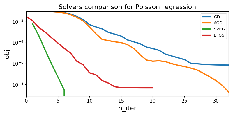
The plot given below compares the distance to the minimum of each solver along iterations, on a logarithmic scale.

../_images/plot_poisson_regression_001.png

Python source code: plot_poisson_regression.py

import numpy as np
import matplotlib.pyplot as plt

from tick.simulation import weights_sparse_gauss
from tick.linear_model import SimuPoisReg, PoissonRegression
from tick.plot import plot_history

n_samples = 50000
n_features = 100
np.random.seed(123)
weight0 = weights_sparse_gauss(n_features, nnz=int(n_features - 1)) / 20.
intercept0 = -0.1
X, y = SimuPoisReg(weight0, intercept0, n_samples=n_samples, verbose=False,
                   seed=123).simulate()

opts = {'verbose': False, 'record_every': 1, 'tol': 1e-8, 'max_iter': 40}

poisson_regressions = [
    PoissonRegression(solver='gd', **opts),
    PoissonRegression(solver='agd', **opts),
    PoissonRegression(solver='svrg', random_state=1234, **opts),
    PoissonRegression(solver='bfgs', **opts)
]

for poisson_regression in poisson_regressions:
    poisson_regression.fit(X, y)

plot_history(poisson_regressions, log_scale=True, dist_min=True)
plt.title('Solvers comparison for Poisson regression', fontsize=16)
plt.tight_layout()

Total running time of the example: 11.26 seconds ( 0 minutes 11.26 seconds)

Mentioned tick classes: