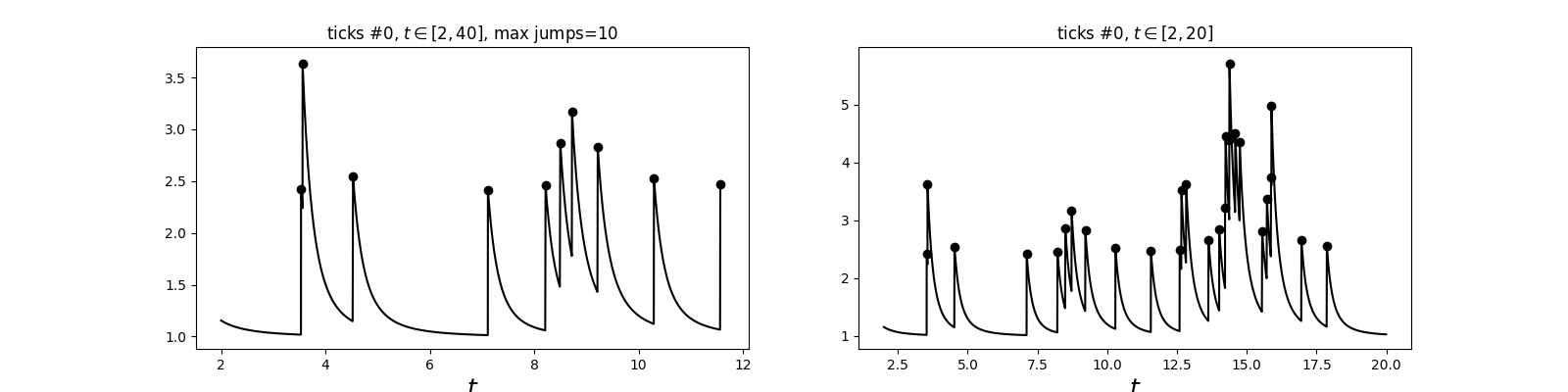
1 dimensional Hawkes process simulation¶

from tick.plot import plot_point_process
from tick.hawkes import SimuHawkes, HawkesKernelSumExp
import matplotlib.pyplot as plt

run_time = 40

hawkes = SimuHawkes(n_nodes=1, end_time=run_time, verbose=False, seed=1398)
kernel = HawkesKernelSumExp([.1, .2, .1], [1., 3., 7.])
hawkes.set_kernel(0, 0, kernel)
hawkes.set_baseline(0, 1.)

dt = 0.01
hawkes.track_intensity(dt)
hawkes.simulate()
timestamps = hawkes.timestamps
intensity = hawkes.tracked_intensity
intensity_times = hawkes.intensity_tracked_times

_, ax = plt.subplots(1, 2, figsize=(16, 4))
plot_point_process(hawkes, n_points=50000, t_min=2, max_jumps=10, ax=ax[0])
plot_point_process(hawkes, n_points=50000, t_min=2, t_max=20, ax=ax[1])