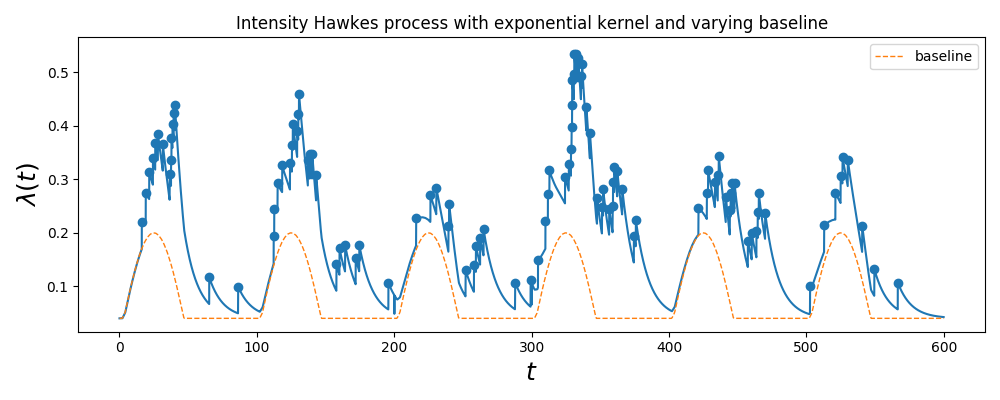
Simulate Hawkes process with non constant baseline
This example simulates a Hawkes process with a non constant, periodic baseline
Python source code: plot_hawkes_varying_baseline_simulation.py
import numpy as np
import matplotlib.pyplot as plt
from tick.base import TimeFunction
from tick.hawkes import SimuHawkesExpKernels
from tick.plot import plot_point_process, qq_plots as _qq_plot
###############################################################################
# instantiate
##############################################################################
period_length = 100
t_values = np.linspace(0, period_length)
y_values = 0.2 * np.maximum(
np.sin(t_values * (2 * np.pi) / period_length), 0.2)
baselines = np.array(
[TimeFunction((t_values, y_values), border_type=TimeFunction.Cyclic)])
decay = 0.1
adjacency = np.array([[0.5]])
hawkes = SimuHawkesExpKernels(adjacency,
decay,
baseline=baselines,
seed=2093,
verbose=False,
)
###############################################################################
# simulate
##############################################################################
period_length = 100
hawkes.track_intensity(0.1)
hawkes.end_time = 6 * period_length
hawkes.simulate()
###############################################################################
# plot intensity
##############################################################################
fig1, ax = plt.subplots(1, 1, figsize=(10, 4))
plot_point_process(hawkes, ax=ax)
t_values = np.linspace(0, hawkes.end_time, 1000)
ax.plot(t_values,
hawkes.get_baseline_values(0, t_values),
label='baseline',
ls='--', lw=1)
ax.set_ylabel("$\lambda(t)$", fontsize=18)
ax.legend()
plt.title("Intensity Hawkes process with exponential kernel and varying "
"baseline")
###############################################################################
# qq plot
##############################################################################
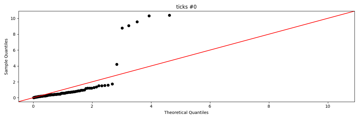
hawkes.store_compensator_values()
fig2 = _qq_plot(hawkes)
###############################################################################
# show
##############################################################################
fig1.tight_layout()
fig2.tight_layout()
plt.show()
Total running time of the example: 0.07 seconds ( 0 minutes 0.07 seconds)
- Mentioned tick classes:
tick.base.TimeFunction.Cyclictick.plot.qq_plots