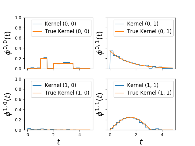
Fit Hawkes random kernels
This Hawkes EM (tick.inference.HawkesEM) algorithm assume that kernels are
piecewise constant. Hence it can fit basically any kernel form. However it
doesn’t scale very well.
It has been originally described in this paper:
Lewis, E., & Mohler, G. (2011). A nonparametric EM algorithm for multiscale Hawkes processes. preprint, 1-16.
Python source code: plot_hawkes_em.py
import numpy as np
import matplotlib.pyplot as plt

from tick.hawkes import (SimuHawkes, HawkesKernelTimeFunc, HawkesKernelExp,
                         HawkesEM)
from tick.base import TimeFunction
from tick.plot import plot_hawkes_kernels

run_time = 30000

t_values1 = np.array([0, 1, 1.5, 2., 3.5], dtype=float)
y_values1 = np.array([0, 0.2, 0, 0.1, 0.], dtype=float)
tf1 = TimeFunction([t_values1, y_values1],
                   inter_mode=TimeFunction.InterConstRight, dt=0.1)
kernel1 = HawkesKernelTimeFunc(tf1)

t_values2 = np.linspace(0, 4, 20)
y_values2 = np.maximum(0., np.sin(t_values2) / 4)
tf2 = TimeFunction([t_values2, y_values2])
kernel2 = HawkesKernelTimeFunc(tf2)

baseline = np.array([0.1, 0.3])

hawkes = SimuHawkes(baseline=baseline, end_time=run_time, verbose=False,
                    seed=2334)

hawkes.set_kernel(0, 0, kernel1)
hawkes.set_kernel(0, 1, HawkesKernelExp(.5, .7))
hawkes.set_kernel(1, 1, kernel2)

hawkes.simulate()

em = HawkesEM(4, kernel_size=16, n_threads=8, verbose=False, tol=1e-3)
em.fit(hawkes.timestamps)

fig = plot_hawkes_kernels(em, hawkes=hawkes, show=False)

for ax in fig.axes:
    ax.set_ylim([0, 1])
plt.show()
Total running time of the example: 0.39 seconds ( 0 minutes 0.39 seconds)
- Mentioned tick classes:
tick.base.TimeFunction.InterConstRight