Hawkes simulation with exotic kernels
Simulation of Hawkes processes with usage of custom kernels
Python source code: plot_hawkes_time_func_simu.py
import matplotlib.pyplot as plt
import numpy as np
from tick.base import TimeFunction
from tick.hawkes import SimuHawkes, HawkesKernelExp, HawkesKernelTimeFunc
from tick.plot import plot_point_process, qq_plots as _qq_plots
###############################################################################
# instantiate
###############################################################################
t_values = np.array([0, 1, 1.5], dtype=float)
y_values = np.array([0, .2, 0], dtype=float)
tf1 = TimeFunction([t_values, y_values],
inter_mode=TimeFunction.InterConstRight, dt=0.1)
kernel_1 = HawkesKernelTimeFunc(tf1)
t_values = np.array([0, .1, 2], dtype=float)
y_values = np.array([0, .4, -0.2], dtype=float)
tf2 = TimeFunction([t_values, y_values], inter_mode=TimeFunction.InterLinear,
dt=0.1)
kernel_2 = HawkesKernelTimeFunc(tf2)
model = SimuHawkes(
kernels=[[kernel_1, kernel_1], [HawkesKernelExp(.07, 4), kernel_2]],
baseline=[1.5, 1.5], verbose=False, seed=23983)
###############################################################################
# simulate
###############################################################################
run_time = 40
dt = 0.01
model.track_intensity(dt)
model.end_time = run_time
model.simulate()
###############################################################################
# plot
###############################################################################
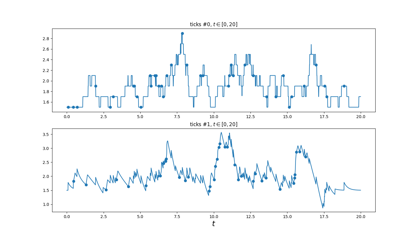
fig1, ax = plt.subplots(model.n_nodes, 1, figsize=(14, 8))
plot_point_process(model, t_max=20, ax=ax)
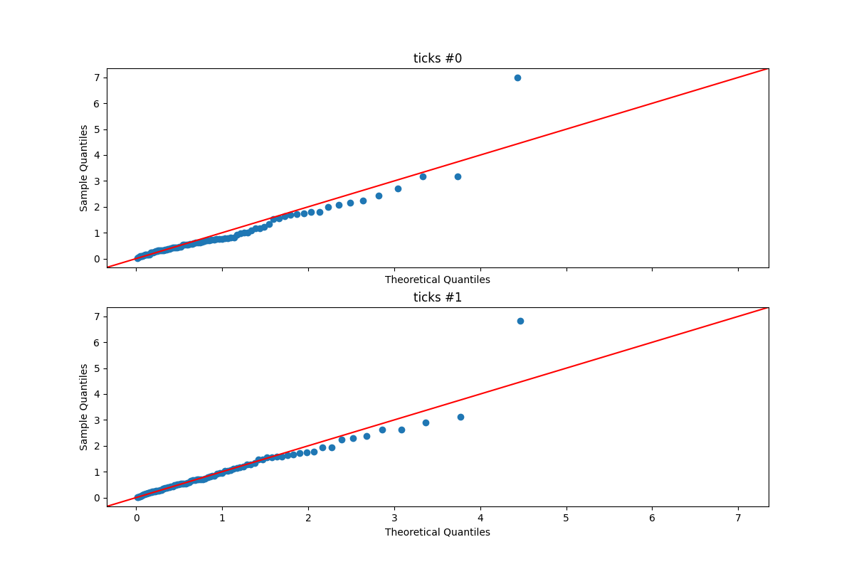
model.store_compensator_values()
fig2 = _qq_plots(model, show=False)
plt.show()
Total running time of the example: 0.26 seconds ( 0 minutes 0.26 seconds)
- Mentioned tick classes:
tick.base.TimeFunction.InterConstRighttick.base.TimeFunction.InterLineartick.plot.qq_plots