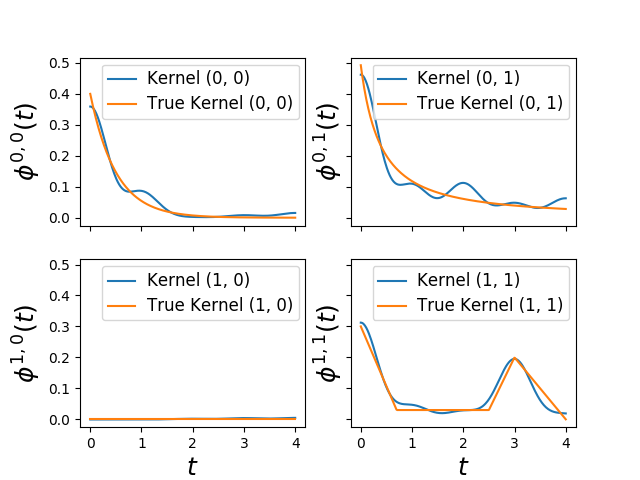
Fit Hawkes with asynchronous causality
This Hawkes (tick.inference.HawkesSumGaussians) algorithm assume
that kernels are parametrized as a sum of gaussians. This can be useful to
determine whether an action will have an effect in a not so near future. For
example if you watch a TV show today you might be stimulated to watch the same
TV show one week later.
I has been originally described in this paper:
Xu, Farajtabar, and Zha (2016, June) in ICML, Learning Granger Causality for Hawkes Processes.

Python source code: plot_hawkes_gaussian_kernels.py
import numpy as np

from tick.plot import plot_hawkes_kernels
from tick.hawkes import (SimuHawkes, SimuHawkesMulti, HawkesKernelExp,
                         HawkesKernelTimeFunc, HawkesKernelPowerLaw,
                         HawkesKernel0, HawkesSumGaussians)

end_time = 1000
n_nodes = 2
n_realizations = 10
n_gaussians = 5

timestamps_list = []

kernel_timefunction = HawkesKernelTimeFunc(
    t_values=np.array([0., .7, 2.5, 3., 4.]),
    y_values=np.array([.3, .03, .03, .2, 0.]))
kernels = [[HawkesKernelExp(.2, 2.),
            HawkesKernelPowerLaw(.2, .5, 1.3)],
           [HawkesKernel0(), kernel_timefunction]]

hawkes = SimuHawkes(baseline=[.5, .2], kernels=kernels, end_time=end_time,
                    verbose=False, seed=1039)

multi = SimuHawkesMulti(hawkes, n_simulations=n_realizations)

multi.simulate()

learner = HawkesSumGaussians(n_gaussians, max_iter=10)
learner.fit(multi.timestamps)

plot_hawkes_kernels(learner, hawkes=hawkes, support=4)
Total running time of the example: 0.95 seconds ( 0 minutes 0.95 seconds)